
Introduction
Hey Everyone! I’m back with anoher tutorial on the Task 2 of thsame virtual experience program. I completed this Virtual Experience Program a month back and I have posted the solutions of Task 1. You should visit that too before continuing this tutorial.
This post is specifically about Task 2 - Experimentation and uplift testing You can view this Virtual Experience Program and enroll for the same.
Through the entire Task 1, I learnt how simple and efficient their solution module is rather than my way of writing code. So, instead I learnt their efficient yet short and simple coding and applied it to Task 2.
So, lets dive straight to the solution.
Load required libraries and datasets
rm(list = ls())
library(data.table)
library(tibble)
library(ggplot2)
library(tidyr)
Load the dataset
data <- fread("QVI_data2.csv")Set themes for plots
theme_set(theme_bw())
theme_update(plot.title = element_text(hjust = 0.5))
Select Control Stores
The client has selected store numbers 77, 86 and 88 as trial stores and want control stores to be established stores that are operational for the entire observation period. We would want to match trial stores to control stores that are similar to the trial store prior to the trial period of Feb 2019 in terms of :
- Monthly overall sales revenue
- Monthly number of customers
- Monthly number of transactions per customer
Let’s first create the metrics of interest and filter to stores that are present throughout the pre-trial period.
#### Calculate these measures over time for each store
#### Add a new month ID column in the data with the format yyyymm.
library(lubridate)
library(tidyverse)
library(dplyr)

monthYear <- format(as.Date(data$DATE),"%Y%m")
data[, YEARMONTH := monthYear]

data$YEARMONTH <- as.numeric(as.character(data$YEARMONTH))

#### Next, we define the measure calculations to use during the analysis.
####For each store and month calculate total sales, number of customers,transactions per customer, chips per customer and the average price per unit.

measureOverTime <- data %>% group_by(STORE_NBR,YEARMONTH) %>% summarise(totSales = sum(TOT_SALES),nCustomers = uniqueN(LYLTY_CARD_NBR),nTxnPerCust = uniqueN(TXN_ID)/uniqueN(LYLTY_CARD_NBR), nChipsPerTxn = sum(PROD_QTY)/uniqueN(TXN_ID), avgPricePerUnit = (sum(TOT_SALES)/sum(PROD_QTY)))


#### Filter to the pre-trial period and stores with full observation periods
storesWithFullObs <- as.data.table(table(measureOverTime$STORE_NBR))
storesWithFullObs <- storesWithFullObs %>% filter(N==12)
storesWithFullObs<-setNames(storesWithFullObs,c("STORE_NBR","N"))


preTrialMeasures <- measureOverTime %>% filter(YEARMONTH < 201902,STORE_NBR %in% storesWithFullObs$STORE_NBR)
Now we need to work out a way of ranking how similar each potential control store is to the trial store. We ca calculate how correlated the performance of each store is to the trial store.
Let’s write a function for this so that we don’t have to calculate this for each trial store and control store pair.
#### Create a function to calculate correlation for a measure, looping through each control store.

#For Sales
trialStore_sales <- preTrialMeasures %>% filter(STORE_NBR ==77)
trialStore_sales <- trialStore_sales %>% select(STORE_NBR,YEARMONTH,totSales,nCustomers)

calCorr <- function(preTrialMeasures,trialStore_sales,trialStoreN){

  calTable = data.table(Store1 = numeric(), Store2 = numeric(), corr_measure = numeric())

  stN <- preTrialMeasures %>% select(STORE_NBR)

  for(i in stN$STORE_NBR){

    contSt <- preTrialMeasures %>% filter(STORE_NBR==i)
    contSt <- contSt %>% select(totSales)

    calMeasure = data.table("Store1" = trialStoreN, "Store2" = i, "corr_measure" = cor(trialStore_sales$totSales,contSt$totSales))

    calTable <- rbind(calTable, calMeasure) }
  return(calTable)

}

##For Customers
calculateCorrelation <- function(preTrialMeasures,trialStore_sales,trialStoreN){

  calTable = data.table(Store1 = numeric(), Store2 = numeric(), corr_measure = numeric())

  stN <- preTrialMeasures %>% select(STORE_NBR)

  for(i in stN$STORE_NBR){

    contSt <- preTrialMeasures %>% filter(STORE_NBR==i)
    contSt <- contSt %>% select(nCustomers)

    calMeasure = data.table("Store1" = trialStoreN, "Store2" = i, "corr_measure" = cor(trialStore_sales$nCustomers,contSt$nCustomers))

    calTable <- rbind(calTable, calMeasure) }
  return(calTable)

}
Apart from correlation, we can also calculate a standardised metric based on the absolute difference between the trial store’s performance and each control store’s performance.
Let’s write a function for this.
#### Create a function to calculate a standardised magnitude distance for a measure, looping through each control store
##Sales
calculateMagnitudeDistance1 <- function(preTrialMeasures,trialStore_sales,trial_storeN){
  calTable = data.table(Store1 = numeric(), Store2 = numeric(), YEARMONTH = numeric(),mag_measure = numeric())

  stN <- preTrialMeasures %>% select(STORE_NBR)

  for(i in stN$STORE_NBR){

    contSt <- preTrialMeasures %>% filter(STORE_NBR==i)
    contSt <- contSt %>% select(totSales)

    calMeasure = data.table("Store1" = trial_storeN, "Store2" = i, "YEARMONTH" = preTrialMeasures$YEARMONTH ,"mag_measure" = abs(trialStore_sales$totSales - contSt$totSales))

    calTable <- rbind(calTable,calMeasure)
    calTable <- unique(calTable)
  }
   return(calTable)
}

###Standardize
standMag1 <- function(magnitude_nSales) {
  minMaxDist <- magnitude_nSales[, .(minDist = min( magnitude_nSales$mag_measure), maxDist = max(magnitude_nSales$mag_measure)), by = c("Store1", "YEARMONTH")]
  distTable <- merge(magnitude_nSales, minMaxDist, by = c("Store1", "YEARMONTH"))
  distTable[, magnitudeMeasure := 1 - (mag_measure - minDist)/(maxDist - minDist)]
  finalDistTable <- distTable[, .(magN_measure = mean(magnitudeMeasure)), by = .(Store1, Store2)]
  return(finalDistTable)
}


##Customers
calculateMagnitudeDistance2 <- function(preTrialMeasures,trialStore_sales,trial_storeN){
  calTable = data.table(Store1 = numeric(), Store2 = numeric(), YEARMONTH = numeric(),mag_measure = numeric())

  stN <- preTrialMeasures %>% select(STORE_NBR)

  for(i in stN$STORE_NBR){

    contSt <- preTrialMeasures %>% filter(STORE_NBR==i)
    contSt <- contSt %>% select(nCustomers)

    calMeasure = data.table("Store1" = trial_storeN, "Store2" = i, "YEARMONTH" = preTrialMeasures$YEARMONTH ,"mag_measure" = abs(trialStore_sales$nCustomers - contSt$nCustomers))

    calTable <- rbind(calTable,calMeasure)
    calTable <- unique(calTable)
  }
   return(calTable)
}

###Standardize
standMag2 <- function(magnitude_nCustomers) {
  minMaxDist <- magnitude_nCustomers[, .(minDist = min( magnitude_nCustomers$mag_measure), maxDist = max(magnitude_nCustomers$mag_measure)), by = c("Store1", "YEARMONTH")]
  distTable <- merge(magnitude_nCustomers, minMaxDist, by = c("Store1", "YEARMONTH"))
  distTable[, magnitudeMeasure := 1 - (mag_measure - minDist)/(maxDist - minDist)]
  finalDistTable <- distTable[, .(magN_measure = mean(magnitudeMeasure)), by = .(Store1, Store2)]
  return(finalDistTable)
}
Now let’s use the functions to find the control stores! We’ll select control stores based on how similar monthly total sales in dollar amounts and monthly number of customers are to the trial stores. So we will need to use our functions to get four scores, two for each of total sales and total customers
#### Use the function you created to calculate correlations against store 77 using total sales and number of customers.
trial_store <- 77
corr_nSales <- calCorr(preTrialMeasures,trialStore_sales,trial_store)
corr_nSales <- unique(corr_nSales)

corr_nCustomers <- calculateCorrelation(preTrialMeasures, trialStore_sales, trial_store )
corr_nCustomers <- unique(corr_nCustomers)

#### Use the functions for calculating magnitude
magnitude_nSales <- calculateMagnitudeDistance1(preTrialMeasures, trialStore_sales, trial_store)
magnitude_nSales <- standMag1(magnitude_nSales)
magnitude_nCustomers <‐ calculateMagnitudeDistance2(preTrialMeasures,trialStore_sales, trial_store)
magnitude_nCustomers <- standMag2(magnitude_nCustomers)
We’ll need to combine the all the scores calculated using our function to create a composite score to rank on.
Let’s take a simple average of the correlation and magnitude scores for each driver. Note that if we consider it more important for the trend of the drivers to be similar, we can increase the weight of the correlation score (a simple average gives a weight of 0.5 to the corr_weight) or if we consider the absolute size of the drivers to be more important, we can lower the weight of the correlation score.
corr_weight <- 0.5

score_nSales <- merge(corr_nSales,magnitude_nSales, by = c("Store1", "Store2"))
score_nSales <- score_nSales %>% mutate(scoreNSales = (score_nSales$corr_measure * corr_weight)+(score_nSales$magN_measure * (1 - corr_weight)))

score_nCustomers <- merge(corr_nCustomers,magnitude_nCustomers, by = c("Store1", "Store2"))
score_nCustomers <- score_nCustomers %>% mutate(scoreNCust = (score_nCustomers$corr_measure * corr_weight)+(score_nCustomers$magN_measure * (1 - corr_weight)))
Now we have a score for each of total number of sales and number of customers. Let’s combine the two via a simple average.
score_Control <- merge(score_nSales,score_nCustomers, by = c("Store1", "Store2"))
score_Control <- score_Control %>% mutate(finalControlScore = (scoreNSales * 0.5) + (scoreNCust * 0.5))
The store with the highest score is then selected as the control store since it is most similar to the trial store.
#### Select control stores based on the highest matching store (closest to 1 but not the store itself, i.e. the second ranked highest store)
control_store <- score_Control[order(-finalControlScore),]
control_store <- control_store$Store2
control_store <- control_store[2]
Now that we have found a control store, let’s check visually if the drivers are indeed similar in the period before the trial.
#### Visual checks on trends based on the drivers

measureOverTimeSales <- as.data.table(measureOverTime)
pastSales <- measureOverTimeSales[, Store_type := ifelse(STORE_NBR == trial_store, "Trial",ifelse(STORE_NBR == control_store,"Control", "Other stores"))][, totSales := mean(totSales), by = c("YEARMONTH","Store_type")][, TransactionMonth := as.Date(paste(YEARMONTH %/%100, YEARMONTH %% 100, 1, sep = "‐"), "%Y‐%m‐%d")][YEARMONTH < 201903 , ]

##Visualize
ggplot(pastSales, aes(TransactionMonth, totSales, color = Store_type)) + geom_line() + labs(x = "Month of Operation", y = "Total Sales", title = "Total Sales by Month")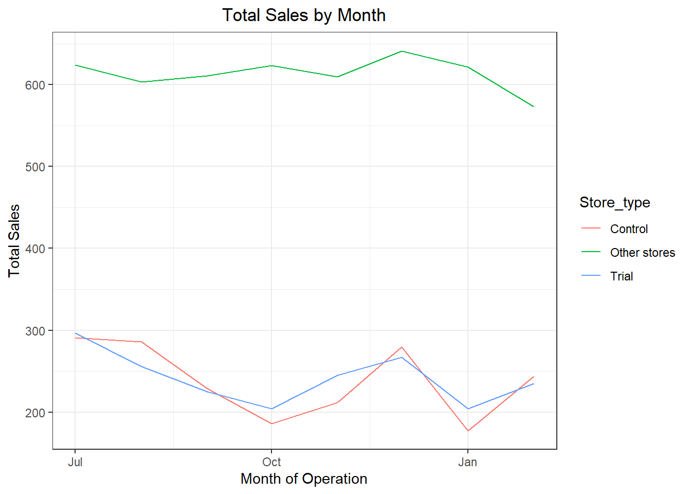
Next, number of Customers
Conduct visual checks on customer count trends by comparing the trial store to the control store and other stores.
measureOverTimeCusts <- as.data.table(measureOverTime)
pastCustomers <- measureOverTimeCusts[, Store_type := ifelse(STORE_NBR == trial_store, "Trial",ifelse(STORE_NBR == control_store,"Control", "Other stores"))][, numberCustomers := mean(nCustomers), by = c("YEARMONTH","Store_type")][, TransactionMonth := as.Date(paste(YEARMONTH %/%100, YEARMONTH %% 100, 1, sep = "‐"), "%Y‐%m‐%d")][YEARMONTH < 201903 ]

###Visualize
ggplot(pastCustomers, aes(TransactionMonth, numberCustomers, color = Store_type)) + geom_line() + labs(x = "Month of Operation", y = "Total Number of Customers", title = "Total Number of Customers by Month")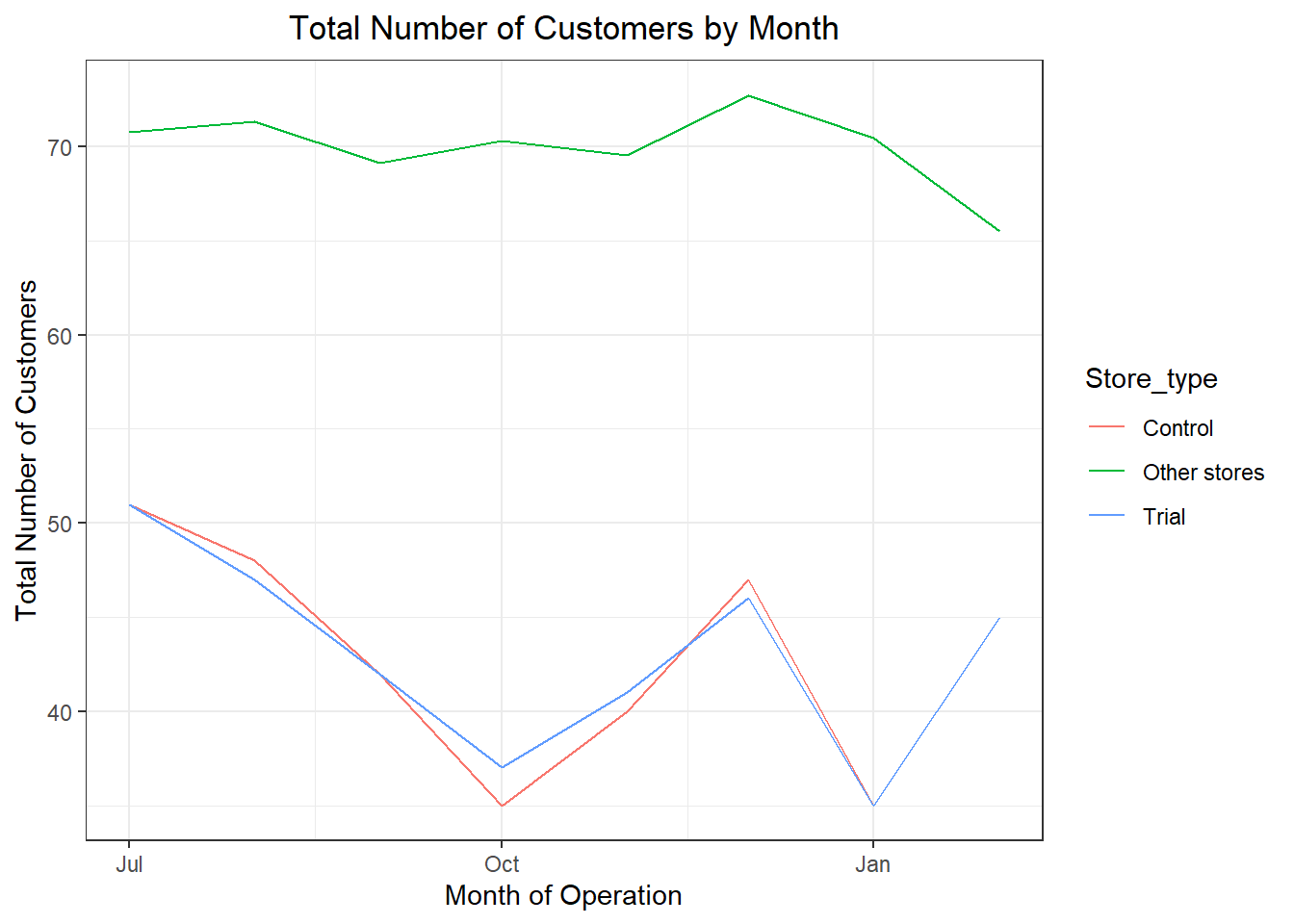
Assessment of Trial
The trial period goes from the start of February 2019 to April 2019. We now want to see if there has been an uplift in overall chip sales.
We’ll start with scaling the control store’s sales to a level similar to control for any differences between the two stores outside of the trial period.
preTrialMeasures <- as.data.table(preTrialMeasures)
scalingFactorForControlSales <- preTrialMeasures[STORE_NBR == trial_store & YEARMONTH < 201902, sum(totSales)]/preTrialMeasures[STORE_NBR == control_store & YEARMONTH < 201902, sum(totSales)]

##Applying the Scaling Factor
measureOverTimeSales <- as.data.table(measureOverTime)
scaledControlSales <- measureOverTimeSales[STORE_NBR == control_store, ][ , controlSales := totSales * scalingFactorForControlSales ]
Now that we have comparable sales figures for the control store, we can calculate the percentage difference between the scaled control sales and the trial store’s sales during the trial period.
 measureOverTime <- as.data.table(measureOverTime)
percentageDiff <- merge(scaledControlSales[, c("YEARMONTH", "controlSales")], measureOverTime[STORE_NBR == trial_store, c("totSales", "YEARMONTH")], by = "YEARMONTH")[ , percentageDiff := abs(controlSales - totSales)/controlSales]
Let’s see if the difference is significant!
#### As our null hypothesis is that the trial period is the same as the pre-trial period, let's take the standard deviation based on the scaled percentage difference in the pre-trial period

stdDev <- sd(percentageDiff[YEARMONTH < 201902, percentageDiff])

#### Note that there are 8 months in the pre-trial period
#### hence 8 - 1 = 7 degrees of freedom
degreesOfFreedom <- 7

#### We will test with a null hypothesis of there being 0 difference between trial and control stores.
#### Calculate the t-values for the trial months.
percentageDiff[ , tvalue := (percentageDiff - 0)/stdDev][ , TransactionMonth := as.Date(paste(YEARMONTH %/% 100, YEARMONTH %% 100, 1, sep = "-"),"%Y-%m-%d")][YEARMONTH < 201905 & YEARMONTH > 201901, .(TransactionMonth, tvalue)]

#### Also,find the 95th percentile of the t distribution with the appropriate degrees of freedom to check whether the hypothesis is statistically significant.

qt(0.95, df = degreesOfFreedom)
We can observe that the t-value is much larger than the 95th percentile value of the t-distribution for March and April i.e. the increase in sales in the trial store in March and April is statistically greater than in the control store.
Let’s create a more visual version of this by plotting the sales of the control store, the sales of the trial stores and the 95th percentile value of sales of the control store.
#measureOverTimeSales <- as.data.table(measureOverTime)

pastSales <- measureOverTimeSales[, Store_type := ifelse(STORE_NBR ==trial_store, "Trial", ifelse(STORE_NBR == control_store,"Control", "Other stores"))][, totSales := mean(totSales), by = c("YEARMONTH","Store_type")][, TransactionMonth := as.Date(paste(YEARMONTH %/% 100, YEARMONTH %% 100, 1, sep = "‐"), "%Y‐%m‐%d")][Store_type %in% c("Trial", "Control"), ]

#pastSales <- as.data.table(pastSales)

### Control Store 95th percentile
pastSales_Controls95 <- pastSales[ Store_type == "Control" , ][, totSales := totSales * (1 + stdDev * 2)][, Store_type := "Control 95th % confidence"]

### Control Store 5th percentile
pastSales_Controls5 <- pastSales[Store_type == "Control" , ][, totSales := totSales * (1 - stdDev * 2)][, Store_type := "Control 5th % confidence"]

trialAssessment <- rbind(pastSales, pastSales_Controls95, pastSales_Controls5)


### Visualize
ggplot(trialAssessment, aes(TransactionMonth, totSales, color = Store_type)) + geom_rect(data = trialAssessment[ YEARMONTH < 201905 & YEARMONTH > 201901 ,], aes(xmin = min(TransactionMonth), xmax = max(TransactionMonth), ymin = 0 , ymax = Inf, color = NULL), show.legend = FALSE) + geom_line() + labs(x = "Month of operation", y = "Total sales", title = "Total sales by month")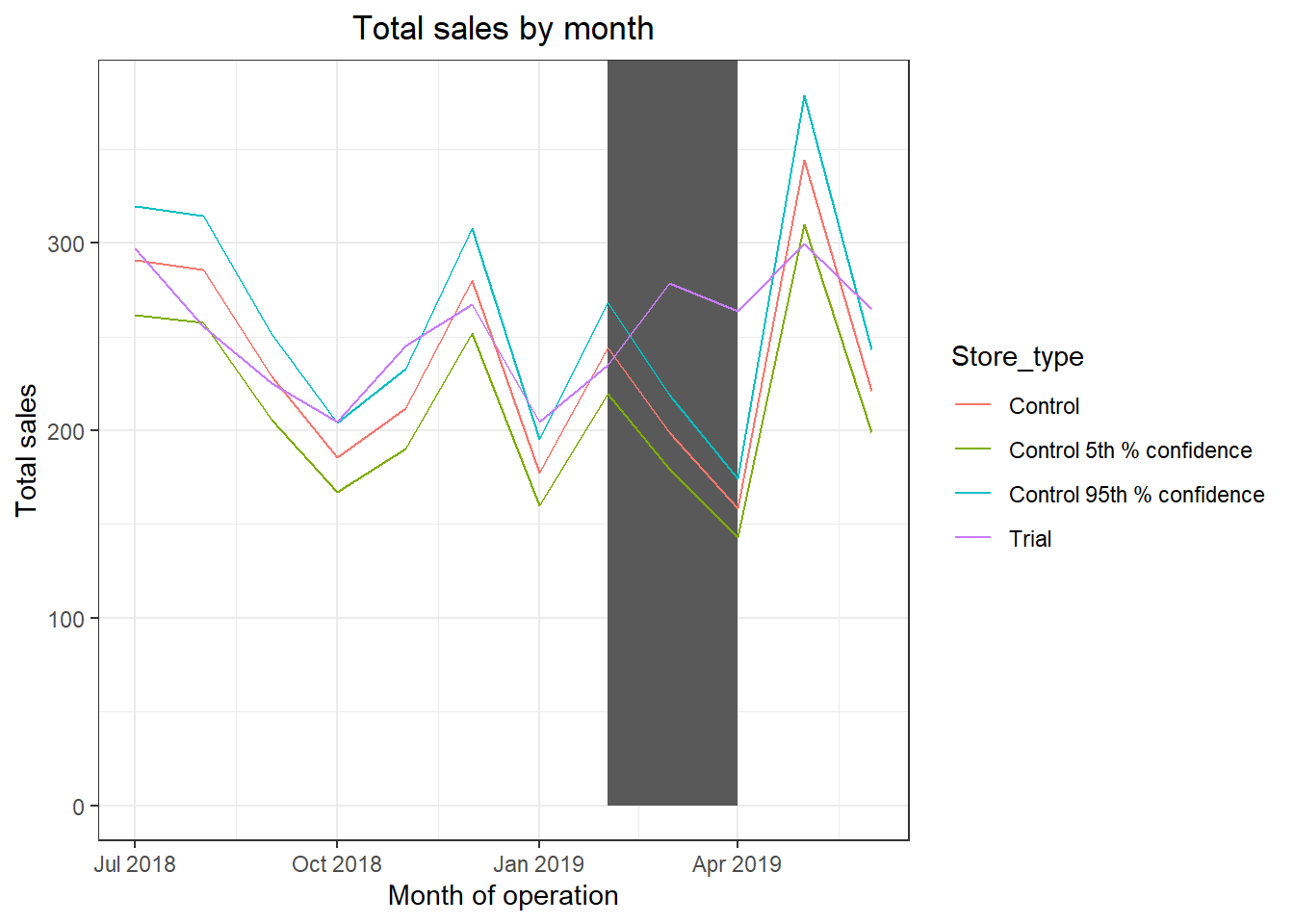
The results show that the trial in store 77 is significantly different to its control store in the trial period as the trial store performance lies outside th 5% to 95% confidence interval of the control store in two of the three trial months.
Let’s have a look at assessing this for number of customers as well.
preTrialMeasures <- as.data.table(preTrialMeasures)

scalingFactorForControlCusts <- preTrialMeasures[STORE_NBR == trial_store & YEARMONTH < 201902, sum(nCustomers)]/preTrialMeasures[STORE_NBR == control_store & YEARMONTH < 201902, sum(nCustomers)]

measureOverTimeCusts <- as.data.table(measureOverTime)

scaledControlCustomers <- measureOverTimeCusts[STORE_NBR == control_store, ][, controlCustomers := nCustomers * scalingFactorForControlCusts][,Store_type := ifelse(STORE_NBR == trial_store, "trial", ifelse(STORE_NBR == control_store,"control","Other Store"))]

###Calculate the % difference between scaled control sales and trial sales
percentageDiff <- merge(scaledControlCustomers[, c("YEARMONTH", "controlCustomers")], measureOverTimeCusts[STORE_NBR == trial_store, c("nCustomers", "YEARMONTH")], by = "YEARMONTH")[ , percentageDiff := abs(controlCustomers - nCustomers)/controlCustomers]
Let’s again see if the difference is significant visually!
#### As our null hypothesis is that the trial period is the same as the pre-trial period, let's take the standard deviation based on the scaled percentage difference in the pre-trial period
stdDev <- sd(percentageDiff[YEARMONTH < 201902 , percentageDiff])

degreesOfFreedom <- 7

#### Trial and control store number of customers
measureOverTimeCusts <- as.data.table(measureOverTime)
pastCustomers <- measureOverTimeCusts[, Store_type := ifelse(STORE_NBR == trial_store, "Trial", ifelse(STORE_NBR == control_store, "Control", "Other stores"))][, nCusts := mean(nCustomers), by = c("YEARMONTH","Store_type")][, TransactionMonth := as.Date(paste(YEARMONTH %/% 100, YEARMONTH %% 100, 1, sep = "‐"), "%Y‐%m‐%d")
][Store_type %in% c("Trial", "Control"), ]

###Control 95th percentile
pastCustomers_Control95 <- pastCustomers[Store_type == "Control",][, nCusts := nCusts * (1 + stdDev * 2)][, Store_type := "Control 95th % confidence interval"]

###Control 5th percentile
pastCustomers_Control5 <- pastCustomers[Store_type == "Control",][, nCusts := nCusts * (1 + stdDev * 2)][, Store_type := "Control 5th % confidence interval"]

trialAssessment <- rbind(pastCustomers,pastCustomers_Control95,pastCustomers_Control5)

###Visualize
ggplot(trialAssessment, aes(TransactionMonth, nCusts, color = Store_type)) + geom_rect(data = trialAssessment[YEARMONTH < 201905 & YEARMONTH > 201901 , ], aes(xmin = min(TransactionMonth), xmax =  max(TransactionMonth), ymin = 0, ymax = Inf, coor = NULL), show.legend = F) + geom_line(aes(linetype = Store_type)) + labs(x = "Month Of Operation", y = "Total Number of Customers", title = "Total Number of Customers by Month")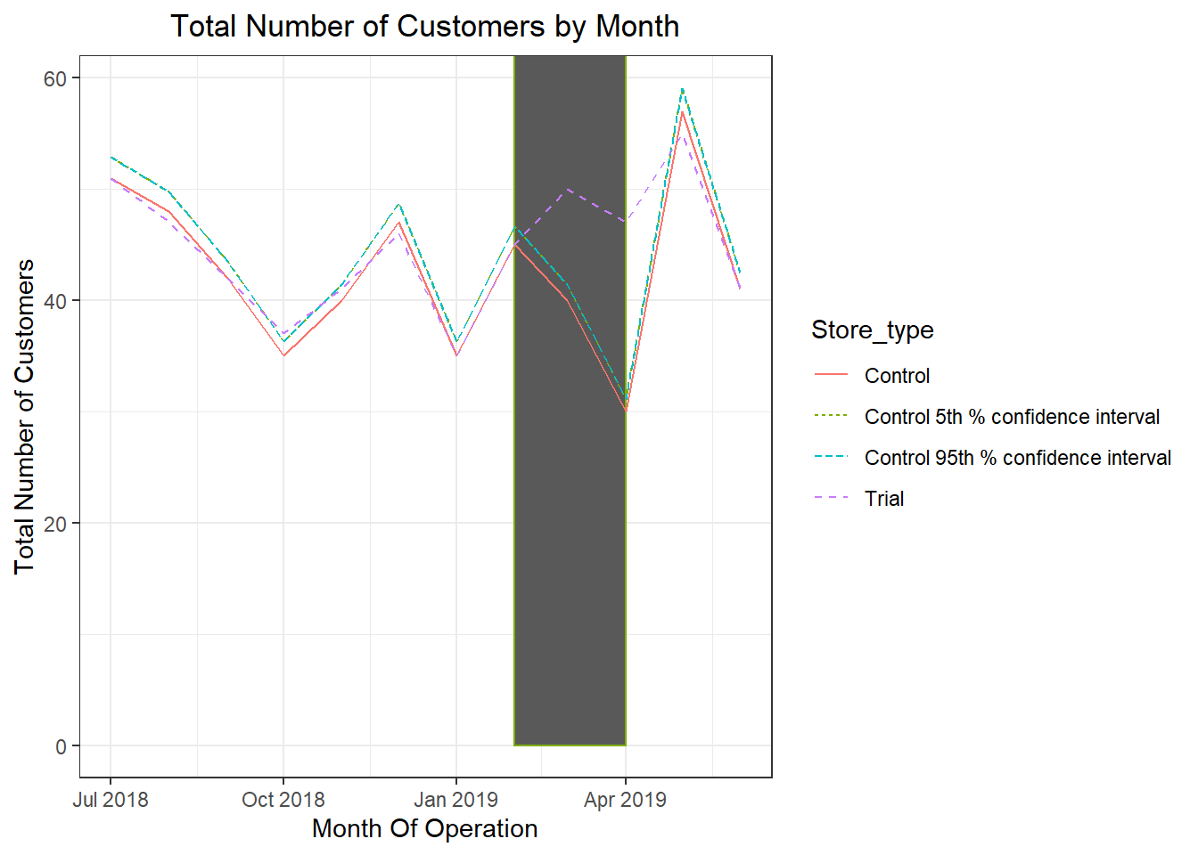
It looks like the number of customers is significantly higher in all of the three months. This seems to suggest that the trial had a significant impact on increasing the number of customers in trial store 86 but as we saw, sales were not significantly higher. We should check with the Category Manager if there were special deals in the trial store that were may have resulted in lower prices, impacting the results.
Let’s repeat finding the control store and assessing the impact of the trial for each of the other two trial stores.
Trial Store 86
data <- as.data.table(data)
measureOverTime <- data[, .(totSales = sum(TOT_SALES), nCustomers = uniqueN(LYLTY_CARD_NBR), nTxnPerCust = uniqueN(TXN_ID)/uniqueN(LYLTY_CARD_NBR), nChipsPerTxn = sum(PROD_QTY)/uniqueN(TXN_ID), avgPricePerUnit = sum(TOT_SALES)/sum(PROD_QTY)), by = c("STORE_NBR", "YEARMONTH")][order(STORE_NBR,YEARMONTH)]

### USe the fucntions for calculating correlation
trial_store <- 86

trialStore_sales <- preTrialMeasures %>% filter(STORE_NBR ==86)
trialStore_sales <- trialStore_sales %>% select(STORE_NBR,YEARMONTH,totSales,nCustomers)

corr_nSales <- calCorr(preTrialMeasures,trialStore_sales,trial_store)
corr_nSales <- unique(corr_nSales)

corr_nCustomers <- calculateCorrelation(preTrialMeasures, trialStore_sales, trial_store )
corr_nCustomers <- unique(corr_nCustomers)

#### Use the functions for calculating magnitude
magnitude_nSales <- calculateMagnitudeDistance1(preTrialMeasures, trialStore_sales, trial_store)
magnitude_nSales <- standMag1(magnitude_nSales)
magnitude_nCustomers <‐ calculateMagnitudeDistance2(preTrialMeasures,trialStore_sales, trial_store)
magnitude_nCustomers <- standMag2(magnitude_nCustomers)

#### Now, create a combined score composed of correlation and magnitude

corr_weight <- 0.5

score_nSales <- merge(corr_nSales,magnitude_nSales, by = c("Store1", "Store2"))
score_nSales <- score_nSales %>% mutate(scoreNSales = (score_nSales$corr_measure * corr_weight)+(score_nSales$magN_measure * (1 - corr_weight)))

score_nCustomers <- merge(corr_nCustomers,magnitude_nCustomers, by = c("Store1", "Store2"))
score_nCustomers <- score_nCustomers %>% mutate(scoreNCust = (score_nCustomers$corr_measure * corr_weight)+(score_nCustomers$magN_measure * (1 - corr_weight)))


#### Finally, combine scores across the drivers using a simple average.

score_Control <- merge(score_nSales,score_nCustomers, by = c("Store1", "Store2"))
score_Control <- score_Control %>% mutate(finalControlScore = (scoreNSales * 0.5) + (scoreNCust * 0.5))


#### Select control stores based on the highest matching store
#### (closest to 1 but not the store itself, i.e. the second ranked highest store)

control_store <- score_Control[order(-finalControlScore),]
control_store <- control_store$Store2
control_store <- control_store[2]
Looks like store 155 will be a control store for trial store 86.
Again, let’s check visually if the drivers are indeed similar in the period before the trial.
We’ll look at total sales first.
measureOverTimeSales <- as.data.table(measureOverTime)
pastSales <- measureOverTimeSales[, Store_type := ifelse(STORE_NBR == trial_store, "Trial", ifelse(STORE_NBR == control_store, "Control", "Other stores"))][, totSales := mean(totSales), by = c("YEARMONTH","Store_type")][, TransactionMonth := as.Date(paste(YEARMONTH %/% 100, YEARMONTH %% 100, 1, sep = "‐"), "%Y‐%m‐%d")][YEARMONTH < 201903 , ]

###Visualize
ggplot(pastSales, aes(TransactionMonth, totSales, color = Store_type)) +
geom_line(aes(linetype = Store_type)) +
labs(x = "Month of operation", y = "Total sales", title = "Total sales by month")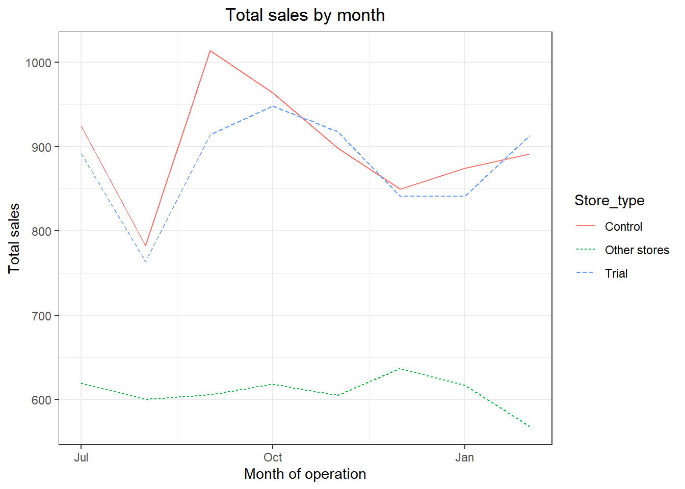
Great, sales are trending in a similar way.
Next, number of customers.
measureOverTimeCusts <- as.data.table(measureOverTime)

pastCustomers <- measureOverTimeCusts[, Store_type := ifelse(STORE_NBR == trial_store, "Trial", ifelse(STORE_NBR == control_store, "Control", "Other stores"))][, nCusts := mean(nCustomers), by = c("YEARMONTH","Store_type")][, TransactionMonth := as.Date(paste(YEARMONTH %/% 100, YEARMONTH %% 100, 1, sep = "‐"), "%Y‐%m‐%d")][YEARMONTH < 201903 ,]

###Visualize
ggplot(pastCustomers, aes(TransactionMonth, nCusts, color = Store_type)) +
geom_line() + labs(x = "Month of operation", y = "Total number of customers", title = "Total number of customers by month")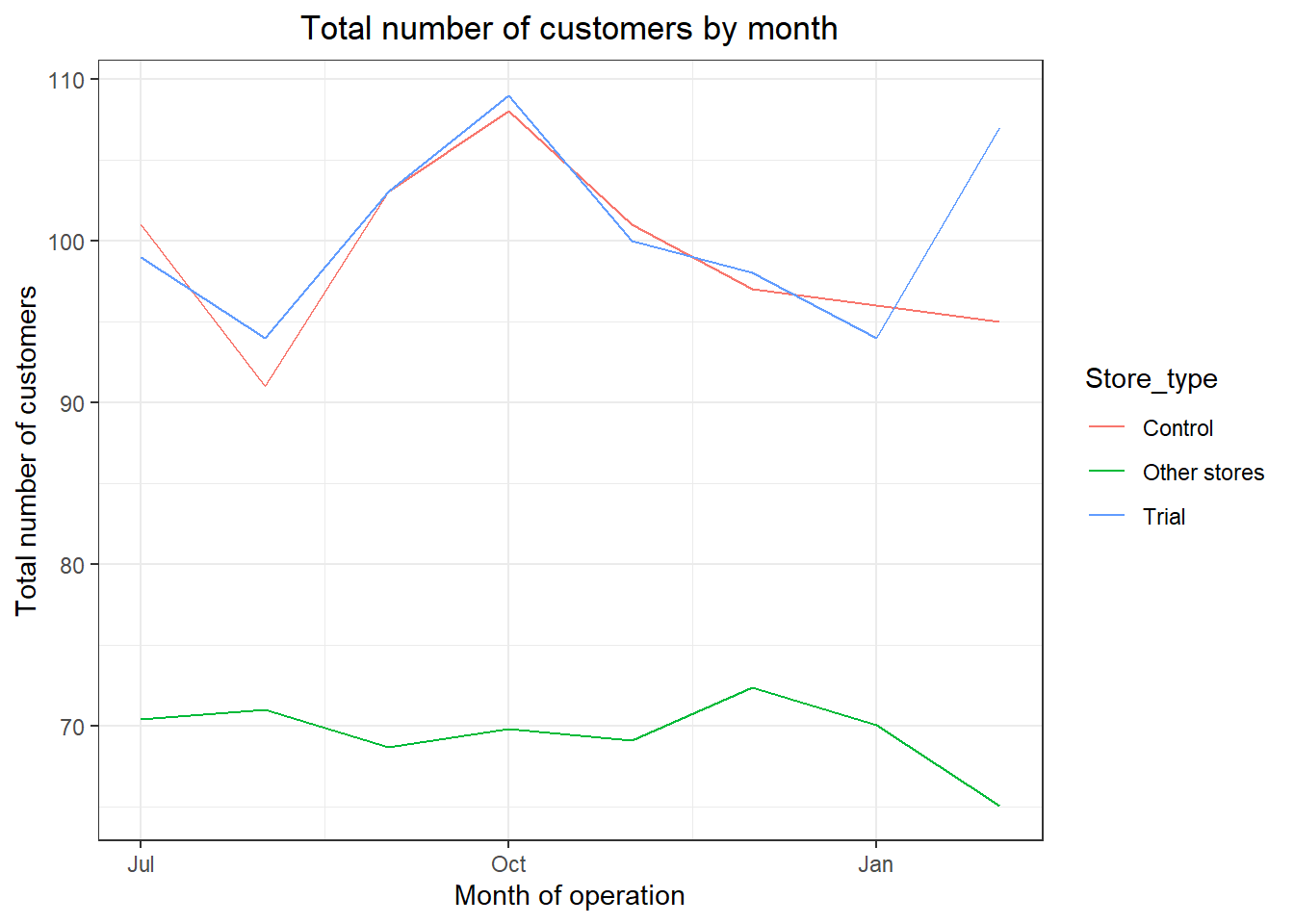
Good, the trend in number of customers is also similar.
Let’s now assess the impact of the trial on sales.
#### Scale pre-trial control sales to match pre-trial trial store sales
scalingFactorForControlSales <- preTrialMeasures[STORE_NBR == trial_store & YEARMONTH < 201902, sum(totSales)]/preTrialMeasures[STORE_NBR == control_store &
YEARMONTH < 201902, sum(totSales)]

#### Apply the scaling factor
measureOverTimeSales <- as.data.table(measureOverTime)
scaledControlSales <- measureOverTimeSales[STORE_NBR == control_store, ][ , controlSales := totSales * scalingFactorForControlSales]

###Calculate the percentage difference between scaled control sales and trial sales

measureOverTime <- as.data.table(measureOverTime)

percentageDiff <-  merge(scaledControlSales[, c("YEARMONTH", "controlSales")], measureOverTime[STORE_NBR == trial_store, c("totSales", "YEARMONTH")], by = "YEARMONTH")[ , percentageDiff := abs(controlSales - totSales)/controlSales]


#### As our null hypothesis is that the trial period is the same as the pre-trial period, let's take the standard deviation based on the scaled percentage difference in the pre-trial period

stdDev <- sd(percentageDiff[YEARMONTH < 201902, percentageDiff])

degreesOfFreedom <- 7

#### Trial and control store total sales
measureOverTimeSales <‐ as.data.table(measureOverTime)
pastSales <‐ measureOverTimeSales[, Store_type := ifelse(STORE_NBR == trial_store, "Trial",
ifelse(STORE_NBR == control_store,"Control", "Other stores")) ][, totSales := mean(totSales), by = c("YEARMONTH","Store_type")][, TransactionMonth := as.Date(paste(YEARMONTH %/% 100, YEARMONTH %% 100, 1, sep = "‐"), "%Y‐%m‐%d")][Store_type %in% c("Trial", "Control"), ]

#### Control store 95th percentile
pastSales_Controls95 <‐ pastSales[Store_type == "Control",][, totSales := totSales * (1 + stdDev * 2)][, Store_type := "Control 95th % confidence interval"]

#### Control store 5th percentile
pastSales_Controls5 <‐ pastSales[Store_type == "Control",][, totSales := totSales * (1 ‐ stdDev * 2)][, Store_type := "Control 5th % confidence interval"]

trialAssessment <‐ rbind(pastSales, pastSales_Controls95, pastSales_Controls5)

#### Plotting these in one nice graph
ggplot(trialAssessment, aes(TransactionMonth, totSales, color = Store_type)) + geom_rect(data = trialAssessment[ YEARMONTH < 201905 & YEARMONTH > 201901 ,], aes(xmin = min(TransactionMonth), xmax = max(TransactionMonth), ymin = 0 ,
ymax = Inf, color = NULL), show.legend = FALSE) + geom_line(aes(linetype = Store_type)) + labs(x = "Month of operation", y = "Total sales", title = "Total sales by month")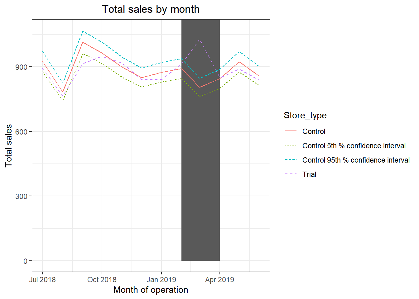
The results show that the trial in store 86 is significantly different to its control store in the trial period as the trial store performance lies outside of the 5% to 95% confidence interval of the control store in two of the three trial months.
Let’s have a look at assessing this for number of customers as well.
scalingFactorForControlCust <‐ preTrialMeasures[STORE_NBR == trial_store & YEARMONTH < 201902, sum(nCustomers)]/preTrialMeasures[STORE_NBR == control_store & YEARMONTH < 201902, sum(nCustomers)]

#### Apply the scaling factor
measureOverTimeCusts <‐ as.data.table(measureOverTime)

scaledControlCustomers <‐ measureOverTimeCusts[STORE_NBR == control_store,][ , controlCustomers := nCustomers * scalingFactorForControlCust][, Store_type := ifelse(STORE_NBR == trial_store, "Trial", ifelse(STORE_NBR == control_store, "Control", "Other stores"))]

#### Calculate the percentage difference between scaled control sales and trial sales
percentageDiff <‐ merge(scaledControlCustomers[, c("YEARMONTH",
"controlCustomers")], measureOverTime[STORE_NBR == trial_store, c("nCustomers", "YEARMONTH")], by = "YEARMONTH")[, percentageDiff :=abs(controlCustomers‐nCustomers)/controlCustomers]


#### As our null hypothesis is that the trial period is the same as the pre‐trial period, let's take the standard deviation based on the scaled percentage difference in the pre‐trial period

stdDev <‐ sd(percentageDiff[YEARMONTH < 201902 , percentageDiff])

degreesOfFreedom <‐ 7 # note that there are 8 months in the pre‐trial period hence 8 ‐ 1 = 7 degrees of freedom

#### Trial and control store number of customers

measureOverTimeCusts <- as.data.table(measureOverTime)

pastCustomers <- measureOverTimeCusts[, Store_type := ifelse(STORE_NBR == trial_store, "Trial", ifelse(STORE_NBR == control_store, "Control", "Other stores"))][, nCusts := mean(nCustomers), by = c("YEARMONTH","Store_type")][, TransactionMonth := as.Date(paste(YEARMONTH %/% 100, YEARMONTH %% 100, 1, sep = "‐"), "%Y‐%m‐%d")][Store_type %in% c("Trial", "Control"), ]

#### Control store 95th percentile
pastCustomers_Controls95 <‐ pastCustomers[Store_type == "Control",][, nCusts := nCusts * (1 + stdDev * 2) ][, Store_type := "Control 95th % confidence interval"]

#### Control store 5th percentile
pastCustomers_Controls5 <‐ pastCustomers[Store_type == "Control",][, nCusts := nCusts * (1 ‐ stdDev * 2)][, Store_type := "Control 5th % confidence interval"]

trialAssessment <‐ rbind(pastCustomers, pastCustomers_Controls95, pastCustomers_Controls5)

#### Visualize
ggplot(trialAssessment, aes(TransactionMonth, nCusts, color = Store_type)) + geom_rect(data = trialAssessment[ YEARMONTH < 201905 & YEARMONTH > 201901 ,], aes(xmin = min(TransactionMonth), xmax = max(TransactionMonth), ymin = 0 ,
ymax = Inf, color = NULL), show.legend = FALSE) + geom_line() +
labs(x = "Month of operation", y = "Total number of customers", title = "Total number of customers by month")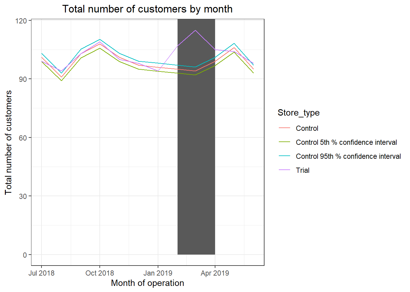
Trial Store 88
data <- as.data.table(data)
measureOverTime <- data[, .(totSales = sum(TOT_SALES), nCustomers = uniqueN(LYLTY_CARD_NBR), nTxnPerCust = uniqueN(TXN_ID)/uniqueN(LYLTY_CARD_NBR), nChipsPerTxn = sum(PROD_QTY)/uniqueN(TXN_ID), avgPricePerUnit = sum(TOT_SALES)/sum(PROD_QTY)), by = c("STORE_NBR", "YEARMONTH")][order(STORE_NBR,YEARMONTH)]

### USe the fucntions for calculating correlation
trial_store <- 88

trialStore_sales <- preTrialMeasures %>% filter(STORE_NBR ==88)
trialStore_sales <- trialStore_sales %>% select(STORE_NBR,YEARMONTH,totSales,nCustomers)

corr_nSales <- calCorr(preTrialMeasures,trialStore_sales,trial_store)
corr_nSales <- unique(corr_nSales)

corr_nCustomers <- calculateCorrelation(preTrialMeasures, trialStore_sales, trial_store )
corr_nCustomers <- unique(corr_nCustomers)

#### Use the functions for calculating magnitude
magnitude_nSales <- calculateMagnitudeDistance1(preTrialMeasures, trialStore_sales, trial_store)
magnitude_nSales <- standMag1(magnitude_nSales)
magnitude_nCustomers <‐ calculateMagnitudeDistance2(preTrialMeasures,trialStore_sales, trial_store)
magnitude_nCustomers <- standMag2(magnitude_nCustomers)

#### Now, create a combined score composed of correlation and magnitude

corr_weight <- 0.5

score_nSales <- merge(corr_nSales,magnitude_nSales, by = c("Store1", "Store2"))
score_nSales <- score_nSales %>% mutate(scoreNSales = (score_nSales$corr_measure * corr_weight)+(score_nSales$magN_measure * (1 -corr_weight)))

score_nCustomers <- merge(corr_nCustomers,magnitude_nCustomers, by = c("Store1", "Store2"))
score_nCustomers <- score_nCustomers %>% mutate(scoreNCust = (score_nCustomers$corr_measure * corr_weight)+(score_nCustomers$magN_measure * (1 - corr_weight)))


#### Finally, combine scores across the drivers using a simple average.

score_Control <- merge(score_nSales,score_nCustomers, by = c("Store1", "Store2"))
score_Control <- score_Control %>% mutate(finalControlScore = (scoreNSales * 0.5) + (scoreNCust * 0.5))


#### Select control stores based on the highest matching store
#### (closest to 1 but not the store itself, i.e. the second ranked highest store)

control_store <- score_Control[order(-finalControlScore),]
control_store <- control_store$Store2
control_store <- control_store[2]
Looks like store 178 will be a control store for trial store 88.
Again, let’s check visually if the drivers are indeed similar in the period before the trial.
We’ll look at total sales first.
measureOverTimeSales <- as.data.table(measureOverTime)
pastSales <- measureOverTimeSales[, Store_type := ifelse(STORE_NBR == trial_store, "Trial", ifelse(STORE_NBR == control_store, "Control", "Other stores"))][, totSales := mean(totSales), by = c("YEARMONTH","Store_type")][, TransactionMonth := as.Date(paste(YEARMONTH %/% 100, YEARMONTH %% 100, 1, sep = "‐"), "%Y‐%m‐%d")][YEARMONTH < 201903 , ]

###Visualize
ggplot(pastSales, aes(TransactionMonth, totSales, color = Store_type)) +
geom_line(aes(linetype = Store_type)) +
labs(x = "Month of operation", y = "Total sales", title = "Total sales by month")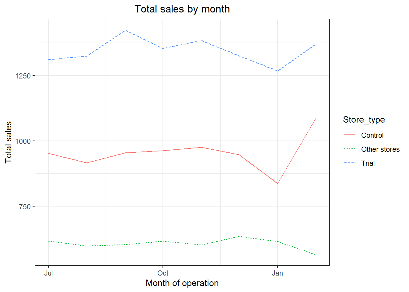
Next, number of customers.
measureOverTimeCusts <- as.data.table(measureOverTime)

pastCustomers <- measureOverTimeCusts[, Store_type := ifelse(STORE_NBR == trial_store, "Trial", ifelse(STORE_NBR == control_store, "Control", "Other stores"))][, nCusts := mean(nCustomers), by = c("YEARMONTH","Store_type")][, TransactionMonth := as.Date(paste(YEARMONTH %/% 100, YEARMONTH %% 100, 1, sep = "‐"), "%Y‐%m‐%d")][YEARMONTH < 201903 ,]

###Visualize
ggplot(pastCustomers, aes(TransactionMonth, nCusts, color = Store_type)) +
geom_line() + labs(x = "Month of operation", y = "Total number of customers", title = "Total number of customers by month")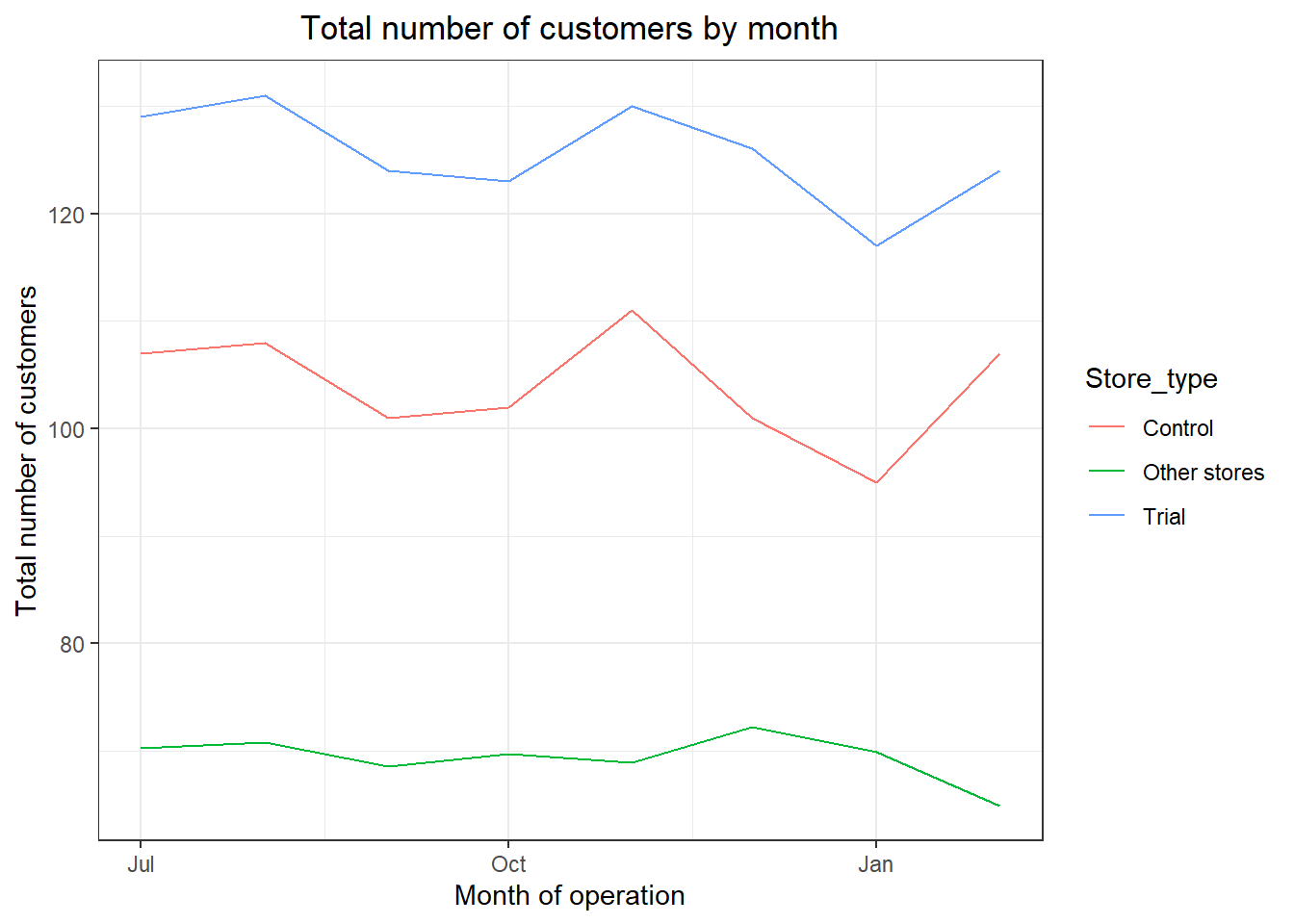
Let’s now assess the impact of the trial on sales.
#### Scale pre-trial control sales to match pre-trial trial store sales
scalingFactorForControlSales <- preTrialMeasures[STORE_NBR == trial_store & YEARMONTH < 201902, sum(totSales)]/preTrialMeasures[STORE_NBR == control_store &
YEARMONTH < 201902, sum(totSales)]

#### Apply the scaling factor
measureOverTimeSales <- as.data.table(measureOverTime)
scaledControlSales <- measureOverTimeSales[STORE_NBR == control_store, ][ , controlSales := totSales * scalingFactorForControlSales]

###Calculate the percentage difference between scaled control sales and trial sales

measureOverTime <- as.data.table(measureOverTime)

percentageDiff <-  merge(scaledControlSales[, c("YEARMONTH", "controlSales")], measureOverTime[STORE_NBR == trial_store, c("totSales", "YEARMONTH")], by = "YEARMONTH")[ , percentageDiff := abs(controlSales - totSales)/controlSales]


#### As our null hypothesis is that the trial period is the same as the pre-trial period, let's take the standard deviation based on the scaled percentage difference in the pre-trial period

stdDev <- sd(percentageDiff[YEARMONTH < 201902, percentageDiff])

degreesOfFreedom <- 7

#### Trial and control store total sales
measureOverTimeSales <‐ as.data.table(measureOverTime)
pastSales <‐ measureOverTimeSales[, Store_type := ifelse(STORE_NBR == trial_store, "Trial",
ifelse(STORE_NBR == control_store,"Control", "Other stores")) ][, totSales := mean(totSales), by = c("YEARMONTH","Store_type")][, TransactionMonth := as.Date(paste(YEARMONTH %/% 100, YEARMONTH %% 100, 1, sep = "‐"), "%Y‐%m‐%d")][Store_type %in% c("Trial", "Control"), ]

#### Control store 95th percentile
pastSales_Controls95 <‐ pastSales[Store_type == "Control",][, totSales := totSales * (1 + stdDev * 2)][, Store_type := "Control 95th % confidence interval"]

#### Control store 5th percentile
pastSales_Controls5 <‐ pastSales[Store_type == "Control",][, totSales := totSales * (1 ‐ stdDev * 2)][, Store_type := "Control 5th % confidence interval"]

trialAssessment <‐ rbind(pastSales, pastSales_Controls95, pastSales_Controls5)

#### Plotting these in one nice graph
ggplot(trialAssessment, aes(TransactionMonth, totSales, color = Store_type)) + geom_rect(data = trialAssessment[ YEARMONTH < 201905 & YEARMONTH > 201901 ,], aes(xmin = min(TransactionMonth), xmax = max(TransactionMonth), ymin = 0 ,
ymax = Inf, color = NULL), show.legend = FALSE) + geom_line(aes(linetype = Store_type)) + labs(x = "Month of operation", y = "Total sales", title = "Total sales by month")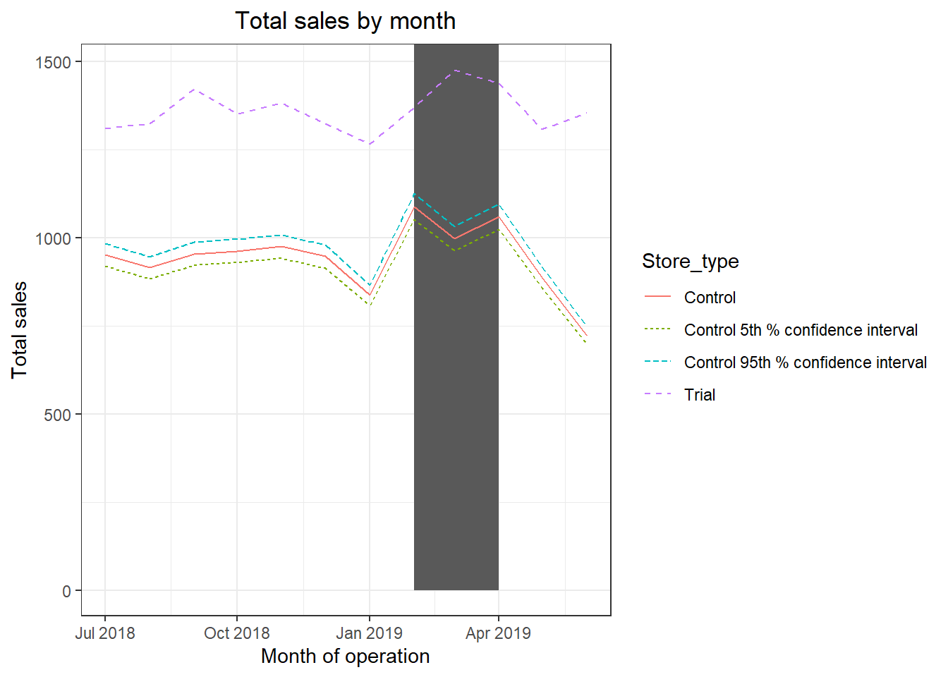
Let’s have a look at assessing this for number of customers as well.
scalingFactorForControlCust <‐ preTrialMeasures[STORE_NBR == trial_store & YEARMONTH < 201902, sum(nCustomers)]/preTrialMeasures[STORE_NBR == control_store & YEARMONTH < 201902, sum(nCustomers)]

#### Apply the scaling factor
measureOverTimeCusts <‐ as.data.table(measureOverTime)

scaledControlCustomers <‐ measureOverTimeCusts[STORE_NBR == control_store,][ , controlCustomers := nCustomers * scalingFactorForControlCust][, Store_type := ifelse(STORE_NBR == trial_store, "Trial", ifelse(STORE_NBR == control_store, "Control", "Other stores"))]

#### Calculate the percentage difference between scaled control sales and trial sales
percentageDiff <‐ merge(scaledControlCustomers[, c("YEARMONTH",
"controlCustomers")], measureOverTime[STORE_NBR == trial_store, c("nCustomers", "YEARMONTH")], by = "YEARMONTH")[, percentageDiff :=abs(controlCustomers‐nCustomers)/controlCustomers]


#### As our null hypothesis is that the trial period is the same as the pre‐trial period, let's take the standard deviation based on the scaled percentage difference in the pre‐trial period

stdDev <‐ sd(percentageDiff[YEARMONTH < 201902 , percentageDiff])

degreesOfFreedom <‐ 7 # note that there are 8 months in the pre‐trial period hence 8 ‐ 1 = 7 degrees of freedom

#### Trial and control store number of customers

measureOverTimeCusts <- as.data.table(measureOverTime)

pastCustomers <- measureOverTimeCusts[, Store_type := ifelse(STORE_NBR == trial_store, "Trial", ifelse(STORE_NBR == control_store, "Control", "Other stores"))][, nCusts := mean(nCustomers), by = c("YEARMONTH","Store_type")][, TransactionMonth := as.Date(paste(YEARMONTH %/% 100, YEARMONTH %% 100, 1, sep = "‐"), "%Y‐%m‐%d")][Store_type %in% c("Trial", "Control"), ]

#### Control store 95th percentile
pastCustomers_Controls95 <‐ pastCustomers[Store_type == "Control",][, nCusts := nCusts * (1 + stdDev * 2) ][, Store_type := "Control 95th % confidence interval"]

#### Control store 5th percentile
pastCustomers_Controls5 <‐ pastCustomers[Store_type == "Control",][, nCusts := nCusts * (1 ‐ stdDev * 2)][, Store_type := "Control 5th % confidence interval"]

trialAssessment <‐ rbind(pastCustomers, pastCustomers_Controls95, pastCustomers_Controls5)

#### Visualize
ggplot(trialAssessment, aes(TransactionMonth, nCusts, color = Store_type)) + geom_rect(data = trialAssessment[ YEARMONTH < 201905 & YEARMONTH > 201901 ,], aes(xmin = min(TransactionMonth), xmax = max(TransactionMonth), ymin = 0 ,
ymax = Inf, color = NULL), show.legend = FALSE) + geom_line() +
labs(x = "Month of operation", y = "Total number of customers", title = "Total number of customers by month")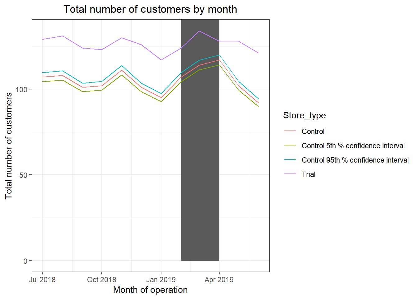
Total number of customers in the trial period for the trial store is significantly higher than the control store for two out of three months, which indicates a positive trial effect.
Conclusion
Good work! We’ve found control stores 233, 155, 178 for trial stores 77, 86 and 88 respectively. The results for trial stores 77 and 86 during the trial period show a significant difference in at least two of the three trial months but this is not the case for trial store 88. We can check with the client if the implementation of the trial was different in trial store 88 but overall, the trial shows a significant increase in sales. Now that we have finished our analysis, we can prepare our presentation to the Category Manager.
Outro
Task 2 was crucial step in analysis so as to identify benchmark stores that would test the impact of the trial store layouts on customer sales. Collation and summarization of all the findings for each store so as to provide a recommendation that we can share outlining the impact on sales during the trial period.
Task 3 is about creating a presentation of all the findings we have gathered through our analysis in Task 1 and 2. I used Google Slides to create my own. You can use the same or any other mode or even the module provided. Task 3 is quite easy but still on demand I can upload the steps to create a presentation for Task 3
Get in touch using any of my social media handles or mail me you queries!
Till then, any feedbacks, queries or recommendations are appreciated on any of my social media handles.
Refer to my Github Profile
Stay tuned for more tutorials!
Thank You!