
Introduction
Hello Everyone! It’s been long since I posted something new. I completed this Virtual Experience Program a month back and thought I could write about the solutions of all the 3 tasks for anyone who might be seeking for the same.
This post is specifically about Task 1 - Data Preparation and Customer Analytics
You are provided initially with the solution modules but still some parts and codes are a bit tough to crack. I did it my way but surely there could be various other solutions to the same problem.
So, lets dive straight to the solutions.
Load the required libraries
library(data.table)
library(ggplot2)
library(ggmosaic)
library(readr)
Examine transaction data
Creating local dataset
To inspect if certain columns are in their specified format for eg. date column is in date format etc.
Also, looking at the description of both the datasets
purchase_beahviour <- as.data.table( read.csv("QVI_purchase_behaviour.csv"))
transaction_data <- as.data.table(readxl::read_xlsx("QVI_transaction_data.xlsx"))

str(purchase_beahviour)
## Classes 'data.table' and 'data.frame': 72637 obs. of 3 variables:
## $ LYLTY_CARD_NBR : int 1000 1002 1003 1004 1005 1007 1009 1010 1011 1012 ...
## $ LIFESTAGE : Factor w/ 7 levels "MIDAGE SINGLES/COUPLES",..: 7 7 6 4 1 7 2 7 4 3 ...
## $ PREMIUM_CUSTOMER: Factor w/ 3 levels "Budget","Mainstream",..: 3 2 1 2 2 1 3 2 2 2 ...
## - attr(*, ".internal.selfref")=<externalptr>str(transaction_data)## Classes 'data.table' and 'data.frame': 264836 obs. of 8 variables:
## $ DATE : num 43390 43599 43605 43329 43330 ...
## $ STORE_NBR : num 1 1 1 2 2 4 4 4 5 7 ...
## $ LYLTY_CARD_NBR: num 1000 1307 1343 2373 2426 ...
## $ TXN_ID : num 1 348 383 974 1038 ...
## $ PROD_NBR : num 5 66 61 69 108 57 16 24 42 52 ...
## $ PROD_NAME : chr "Natural Chip Compny SeaSalt175g" "CCs Nacho Cheese 175g" "Smiths Crinkle Cut Chips Chicken 170g" "Smiths Chip Thinly S/Cream&Onion 175g" ...
## $ PROD_QTY : num 2 3 2 5 3 1 1 1 1 2 ...
## $ TOT_SALES : num 6 6.3 2.9 15 13.8 5.1 5.7 3.6 3.9 7.2 ...
## - attr(*, ".internal.selfref")=<externalptr>EDA (done alreasy using str())
changes!
We saw that the date format is in numeric format which is wrong so we convert it to the date format as shown below
transaction_data$DATE <- as.Date(transaction_data$DATE,origin = "1899-12-30")Now dates are in the right format
Examine PROD_NAME
Generating summary of the PROD_NAME column
#head(transaction_data$PROD_NAME)
transaction_data[, .N, PROD_NAME]
## PROD_NAME N
## 1: Natural Chip Compny SeaSalt175g 1468
## 2: CCs Nacho Cheese 175g 1498
## 3: Smiths Crinkle Cut Chips Chicken 170g 1484
## 4: Smiths Chip Thinly S/Cream&Onion 175g 1473
## 5: Kettle Tortilla ChpsHny&Jlpno Chili 150g 3296
## ---
## 110: Red Rock Deli Chikn&Garlic Aioli 150g 1434
## 111: RRD SR Slow Rst Pork Belly 150g 1526
## 112: RRD Pc Sea Salt 165g 1431
## 113: Smith Crinkle Cut Bolognese 150g 1451
## 114: Doritos Salsa Mild 300g 1472Warning~ Most of the products in PROD_NAME are chips but others may or may not exist.
changes! Looks like we are definitely looking at potato chips but how can we check that these are all chips? We can do some basic text analysis by summarising the individual words in the product name.
#### Examine the words in PROD_NAME to see if there are any incorrect entries
#### such as products that are not chips
productWords <- data.table(unlist(strsplit(unique(transaction_data[, PROD_NAME]), "
")))
setnames(productWords, 'words')
As we are only interested in words that will tell us if the product is chips or not, let’s remove all words with digits and special characters such as ‘&’ from our set of product words. We can do this using grepl().
library(stringr)
library(stringi)

#### Removing special characters
productWords$words <- str_replace_all(productWords$words,"[[:punct:]]"," ")


#### Removing digits
productWords$words <- str_replace_all(productWords$words,"[0-9]"," ")
productWords$words <- str_replace_all(productWords$words,"[gG]"," ")

#### Let's look at the most common words by counting the number of times a word appears and
wordsSep <- strsplit(productWords$words," ")
words.freq<-table(unlist(wordsSep))

#### sorting them by this frequency in order of highest to lowest frequency
words.freq <-  as.data.frame(words.freq)
words.freq <- words.freq[order(words.freq$Freq, decreasing = T),]

words.freq
## Var1 Freq
## 1 732
## 37 Chips 21
## 164 Smiths 16
## 55 Crinkle 14
## 62 Cut 14
## 92 Kettle 13
## 26 Cheese 12
## 152 Salt 12
## 122 Ori 11
## 85 inal 10
## 34 Chip 9
## 68 Doritos 9
## 151 Salsa 9
## 29 Chicken 8
## 52 Corn 8
## 54 Cream 8
## 93 les 8
## 135 Prin 8
## 147 RRD 8
## 32 Chilli 7
## 204 Vine 7
## 209 WW 7
## 4 ar 6
## 156 Sea 6
## 168 Sour 6
## 57 Crisps 5
## 192 Thinly 5
## 193 Thins 5
## 38 Chives 4
## 65 Deli 4
## 86 Infuzions 4
## 95 Lime 4
## 110 Natural 4
## 139 Red 4
## 146 Rock 4
## 185 Supreme 4
## 186 Sweet 4
## 13 BBQ 3
## 22 CCs 3
## 49 Cobs 3
## 66 Dip 3
## 69 El 3
## 94 Li 3
## 103 Mild 3
## 116 Old 3
## 118 Onion 3
## 124 Paso 3
## 129 Popd 3
## 159 Sensations 3
## 171 Soy 3
## 188 Swt 3
## 196 Tomato 3
## 197 Tortilla 3
## 198 Tostitos 3
## 200 Twisties 3
## 208 Woolworths 3
## 3 And 2
## 6 arlic 2
## 19 Bur 2
## 27 Cheetos 2
## 28 Cheezels 2
## 35 ChipCo 2
## 46 Chs 2
## 70 er 2
## 74 French 2
## 78 Honey 2
## 84 htly 2
## 100 Medium 2
## 109 Nacho 2
## 132 Potato 2
## 137 r 2
## 138 rain 2
## 142 Rin 2
## 143 rn 2
## 149 s 2
## 150 S 2
## 154 Salted 2
## 163 Smith 2
## 169 SourCream 2
## 178 SR 2
## 189 Tan 2
## 191 Thai 2
## 201 Tyrrells 2
## 205 Waves 2
## 210 y 2
## 2 Aioli 1
## 5 arden 1
## 7 Ba 1
## 8 Bacon 1
## 9 Balls 1
## 10 Barbecue 1
## 11 Barbeque 1
## 12 Basil 1
## 14 Belly 1
## 15 Bi 1
## 16 Bolo 1
## 17 Box 1
## 18 Btroot 1
## 20 Camembert 1
## 21 camole 1
## 23 Chckn 1
## 24 Ched 1
## 25 Cheddr 1
## 30 Chikn 1
## 31 Chili 1
## 33 Chimuchurri 1
## 36 Chipotle 1
## 39 Chli 1
## 40 Chlli 1
## 41 Chnky 1
## 42 Chp 1
## 43 ChpsBtroot 1
## 44 ChpsFeta 1
## 45 ChpsHny 1
## 47 Chutny 1
## 48 Co 1
## 50 Coconut 1
## 51 Compny 1
## 53 Crackers 1
## 56 Crips 1
## 58 Crm 1
## 59 Crn 1
## 60 Crnchers 1
## 61 Crnkle 1
## 63 CutSalt 1
## 64 D 1
## 67 Dorito 1
## 71 Fi 1
## 72 Flavour 1
## 73 Frch 1
## 75 FriedChicken 1
## 76 Fries 1
## 77 Herbs 1
## 79 Hony 1
## 80 Hot 1
## 81 Hrb 1
## 82 ht 1
## 83 Ht 1
## 87 Infzns 1
## 88 inl 1
## 89 Jalapeno 1
## 90 Jam 1
## 91 Jlpno 1
## 96 Mac 1
## 97 Man 1
## 98 Maple 1
## 99 Med 1
## 101 Mexican 1
## 102 Mexicana 1
## 104 Mozzarella 1
## 105 Mstrd 1
## 106 Mystery 1
## 107 Mzzrlla 1
## 108 N 1
## 111 NCC 1
## 112 nese 1
## 113 nl 1
## 114 o 1
## 115 Of 1
## 117 Onin 1
## 119 OnionDip 1
## 120 OnionStacked 1
## 121 Or 1
## 123 Papadums 1
## 125 Pc 1
## 126 Pepper 1
## 127 Pesto 1
## 128 Plus 1
## 130 Pork 1
## 131 Pot 1
## 133 PotatoMix 1
## 134 Prawn 1
## 136 Puffs 1
## 140 Rib 1
## 141 Ricotta 1
## 144 rnWves 1
## 145 Roast 1
## 148 Rst 1
## 153 saltd 1
## 155 Sauce 1
## 157 SeaSalt 1
## 158 Seasonedchicken 1
## 160 Siracha 1
## 161 Slow 1
## 162 Slt 1
## 165 Smoked 1
## 166 Sna 1
## 167 Snbts 1
## 170 Southern 1
## 172 Sp 1
## 173 Spce 1
## 174 Spcy 1
## 175 Spicy 1
## 176 Splash 1
## 177 Sr 1
## 179 Stacked 1
## 180 Steak 1
## 181 Sthrn 1
## 182 Strws 1
## 183 Style 1
## 184 Sunbites 1
## 187 SweetChili 1
## 190 Tasty 1
## 194 Tmato 1
## 195 Tom 1
## 199 Truffle 1
## 202 Ve 1
## 203 Vin 1
## 206 Whl 1
## 207 Whle 1We saw that we have whitespace maximum number of times and the second most occuring word is chips
Remove salsa products
changes! There are salsa products in the dataset but we are only interested in the chips category, so let’s remove these.
transaction_data[, SALSA := grepl("salsa", tolower(PROD_NAME))]
transaction_data <- transaction_data[SALSA == FALSE, ][, SALSA := NULL]
Next, we can use summary() to check summary statistics such as mean, min and max
values for each feature to see if there are any obvious outliers in the data and if
there are any nulls in any of the columns (NA's : number of nulls will appear in
the output if there are any nulls).
summary(transaction_data)## DATE STORE_NBR LYLTY_CARD_NBR TXN_ID
## Min. :2018-07-01 Min. : 1.0 Min. : 1000 Min. : 1
## 1st Qu.:2018-09-30 1st Qu.: 70.0 1st Qu.: 70015 1st Qu.: 67569
## Median :2018-12-30 Median :130.0 Median : 130367 Median : 135183
## Mean :2018-12-30 Mean :135.1 Mean : 135531 Mean : 135131
## 3rd Qu.:2019-03-31 3rd Qu.:203.0 3rd Qu.: 203084 3rd Qu.: 202654
## Max. :2019-06-30 Max. :272.0 Max. :2373711 Max. :2415841
## PROD_NBR PROD_NAME PROD_QTY TOT_SALES
## Min. : 1.00 Length:246742 Min. : 1.000 Min. : 1.700
## 1st Qu.: 26.00 Class :character 1st Qu.: 2.000 1st Qu.: 5.800
## Median : 53.00 Mode :character Median : 2.000 Median : 7.400
## Mean : 56.35 Mean : 1.908 Mean : 7.321
## 3rd Qu.: 87.00 3rd Qu.: 2.000 3rd Qu.: 8.800
## Max. :114.00 Max. :200.000 Max. :650.000There are no nulls in the columns but product quantity appears to have an outlier which we should investigate further. Let’s investigate further the case where 200 packets of chips are bought in one transaction.
library(tidyverse)
library(dplyr)

prod_qty_200 <- transaction_data %>% filter(PROD_QTY==200)
There are two transactions where 200 packets of chips are bought in one transaction and both of these transactions were by the same customer.
Let’s see if the customer has had other transactions
is_it_same_customer <- transaction_data %>% filter(LYLTY_CARD_NBR == 226000) It looks like this customer has only had the two transactions over the year and is not an ordinary retail customer. The customer might be buying chips for commercial purposes instead. We’ll remove this loyalty card number from further analysis.
Removing this customer from the list
transaction_data <- transaction_data[!(transaction_data$LYLTY_CARD_NBR == 226000)]Re-examine transaction data
summary(transaction_data)## DATE STORE_NBR LYLTY_CARD_NBR TXN_ID
## Min. :2018-07-01 Min. : 1.0 Min. : 1000 Min. : 1
## 1st Qu.:2018-09-30 1st Qu.: 70.0 1st Qu.: 70015 1st Qu.: 67569
## Median :2018-12-30 Median :130.0 Median : 130367 Median : 135182
## Mean :2018-12-30 Mean :135.1 Mean : 135530 Mean : 135130
## 3rd Qu.:2019-03-31 3rd Qu.:203.0 3rd Qu.: 203083 3rd Qu.: 202652
## Max. :2019-06-30 Max. :272.0 Max. :2373711 Max. :2415841
## PROD_NBR PROD_NAME PROD_QTY TOT_SALES
## Min. : 1.00 Length:246740 Min. :1.000 Min. : 1.700
## 1st Qu.: 26.00 Class :character 1st Qu.:2.000 1st Qu.: 5.800
## Median : 53.00 Mode :character Median :2.000 Median : 7.400
## Mean : 56.35 Mean :1.906 Mean : 7.316
## 3rd Qu.: 87.00 3rd Qu.:2.000 3rd Qu.: 8.800
## Max. :114.00 Max. :5.000 Max. :29.500That’s better. Now, let’s look at the number of transaction lines over time to see if there are any obvious data issues such as missing data.
Count the number of transactions by date
countByDate <- count(transaction_data, transaction_data$DATE)
countByDate
## transaction_data$DATE n
## 1: 2018-07-01 663
## 2: 2018-07-02 650
## 3: 2018-07-03 674
## 4: 2018-07-04 669
## 5: 2018-07-05 660
## ---
## 360: 2019-06-26 657
## 361: 2019-06-27 669
## 362: 2019-06-28 673
## 363: 2019-06-29 703
## 364: 2019-06-30 704nrow(countByDate)## [1] 364summary(countByDate)## transaction_data$DATE n
## Min. :2018-07-01 Min. :607.0
## 1st Qu.:2018-09-29 1st Qu.:658.0
## Median :2018-12-30 Median :674.0
## Mean :2018-12-30 Mean :677.9
## 3rd Qu.:2019-03-31 3rd Qu.:694.2
## Max. :2019-06-30 Max. :865.0There’s only 364 rows, meaning only 364 dates which indicates a missing date. Let’s create a sequence of dates from 1 Jul 2018 to 30 Jun 2019 and use this to create a chart of number of transactions over time to find the missing date.
Create a sequence of dates and join this the count of transactions by date
transaction_by_day <- transaction_data[order(DATE),]Setting plot themes to format graphs
theme_set(theme_bw())
theme_update(plot.title = element_text(hjust = 0.5))
Plot transactions over time
transOverTime <-ggplot(countByDate, aes(x = countByDate$`transaction_data$DATE`, y = countByDate$n)) +
 geom_line() +
 labs(x = "Day", y = "Number of transactions", title = "Transactions over time") +
 scale_x_date(breaks = "1 month") +
 theme(axis.text.x = element_text(angle = 90, vjust = 0.5))

transOverTime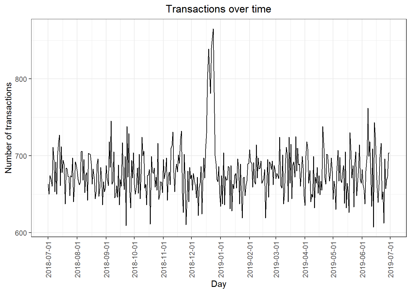
We can see that there is an increase in purchases in December and a break in late December. Let’s zoom in on this.
Filter to December and look at individual days
filterData <- countByDate[countByDate$`transaction_data$DATE` >= "2018-12-01" & countByDate$`transaction_data$DATE` <= "2018-12-31"]

ggplot(filterData, aes(x = filterData$`transaction_data$DATE`, y = filterData$n)) +
 geom_line() +
 labs(x = "Day", y = "Number of transactions", title = "Transactions in December") +
 scale_x_date(breaks = "1 day") +
 theme(axis.text.x = element_text(angle = 90, vjust = 0.5))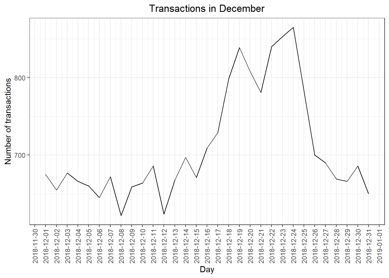
We can see that the increase in sales occurs in the lead-up to Christmas and that there are zero sales on Christmas day itself. This is due to shops being closed on Christmas day.
Now that we are satisfied that the data no longer has outliers, we can move on to creating other features such as brand of chips or pack size from PROD_NAME. We will start with pack size.
Pack size
A new column PACK SIZE added to the data frame transaction_data
#### We can work this out by taking the digits that are in PROD_NAME
transaction_data[, PACK_SIZE := parse_number(PROD_NAME)]

#### Let's check if the pack sizes look sensible
df_packSizeVsTransactions <- transaction_data[, .N, PACK_SIZE][order(PACK_SIZE)]

df_packSizeVsTransactions
## PACK_SIZE N
## 1: 70 1507
## 2: 90 3008
## 3: 110 22387
## 4: 125 1454
## 5: 134 25102
## 6: 135 3257
## 7: 150 40203
## 8: 160 2970
## 9: 165 15297
## 10: 170 19983
## 11: 175 66390
## 12: 180 1468
## 13: 190 2995
## 14: 200 4473
## 15: 210 6272
## 16: 220 1564
## 17: 250 3169
## 18: 270 6285
## 19: 330 12540
## 20: 380 6416The largest size is 380g and the smallest size is 70g - seems sensible!
Let’s plot a histogram of PACK_SIZE since we know that it is a categorical variable and not a continuous variable even though it is numeric.
#ggplot(df_packSizeVsTransactions, aes(x = df_packSizeVsTransactions$PACK_SIZE, y = df_packSizeVsTransactions$N)) +
# geom_line() +
 #labs(x = "Pack Sizes", y = "Number of transactions", title = "Transactions #over time") + scale_x_continuous(breaks = seq(70,390,20)) +
 #theme(axis.text.x = element_text(angle = 90, vjust = 0.5))

hist(transaction_data[, PACK_SIZE])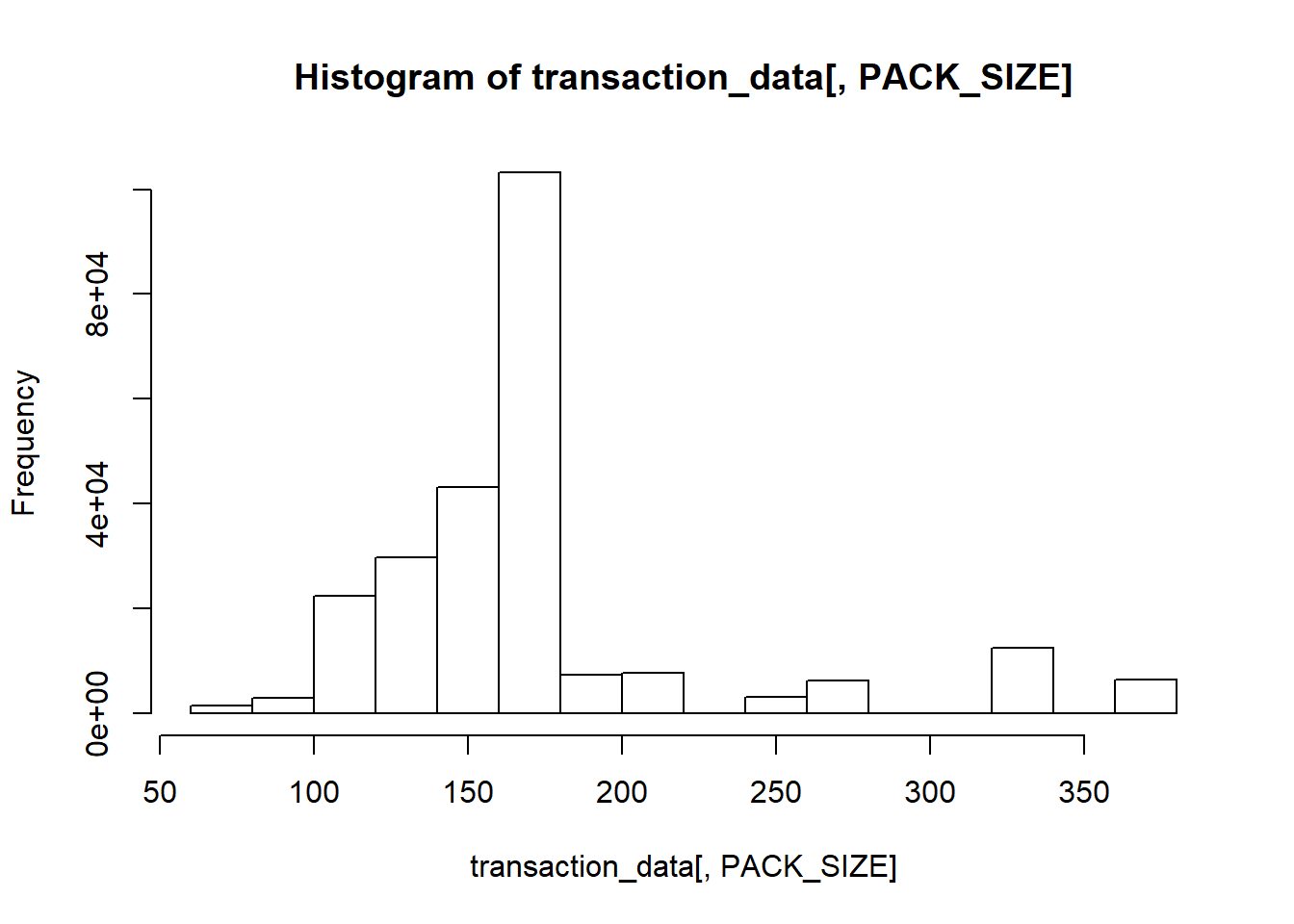
Pack sizes created look reasonable.
Brands
Now to create brands, we can use the first word in PROD_NAME to work out the brand name…
#Create a column which contains the brand of the product, by extracting it from the product name.


transaction_data$BRAND <- gsub("([A-Za-z]+).*", "\\1", transaction_data$PROD_NAME)

transaction_data[, .N, by = BRAND][order(‐N)]
## BRAND N
## 1: Kettle 41288
## 2: Smiths 27390
## 3: Pringles 25102
## 4: Doritos 22041
## 5: Thins 14075
## 6: RRD 11894
## 7: Infuzions 11057
## 8: WW 10320
## 9: Cobs 9693
## 10: Tostitos 9471
## 11: Twisties 9454
## 12: Tyrrells 6442
## 13: Grain 6272
## 14: Natural 6050
## 15: Cheezels 4603
## 16: CCs 4551
## 17: Red 4427
## 18: Dorito 3183
## 19: Infzns 3144
## 20: Smith 2963
## 21: Cheetos 2927
## 22: Snbts 1576
## 23: Burger 1564
## 24: Woolworths 1516
## 25: GrnWves 1468
## 26: Sunbites 1432
## 27: NCC 1419
## 28: French 1418
## BRAND NSome of the brand names look like they are of the same brands - such as RED and RRD, which are both Red Rock Deli chips. Let’s combine these together.
Clean brand names
transaction_data[BRAND == "RED", BRAND := "RRD"]
transaction_data[BRAND == "SNBTS", BRAND := "SUNBITES"]
transaction_data[BRAND == "INFZNS", BRAND := "INFUZIONS"]
transaction_data[BRAND == "WW", BRAND := "WOOLWORTHS"]
transaction_data[BRAND == "SMITH", BRAND := "SMITHS"]
transaction_data[BRAND == "NCC", BRAND := "NATURAL"]
transaction_data[BRAND == "DORITO", BRAND := "DORITOS"]
transaction_data[BRAND == "GRAIN", BRAND := "GRNWVES"]


###Check again
transaction_data[, .N, by = BRAND][order(BRAND)]
## BRAND N
## 1: Burger 1564
## 2: CCs 4551
## 3: Cheetos 2927
## 4: Cheezels 4603
## 5: Cobs 9693
## 6: Dorito 3183
## 7: Doritos 22041
## 8: French 1418
## 9: Grain 6272
## 10: GrnWves 1468
## 11: Infuzions 11057
## 12: Infzns 3144
## 13: Kettle 41288
## 14: NATURAL 1419
## 15: Natural 6050
## 16: Pringles 25102
## 17: RRD 11894
## 18: Red 4427
## 19: Smith 2963
## 20: Smiths 27390
## 21: Snbts 1576
## 22: Sunbites 1432
## 23: Thins 14075
## 24: Tostitos 9471
## 25: Twisties 9454
## 26: Tyrrells 6442
## 27: WOOLWORTHS 10320
## 28: Woolworths 1516
## BRAND NExamining customer data
Now that we are happy with the transaction dataset, let’s have a look at the customer dataset.
summary(purchase_beahviour)## LYLTY_CARD_NBR LIFESTAGE PREMIUM_CUSTOMER
## Min. : 1000 MIDAGE SINGLES/COUPLES: 7275 Budget :24470
## 1st Qu.: 66202 NEW FAMILIES : 2549 Mainstream:29245
## Median : 134040 OLDER FAMILIES : 9780 Premium :18922
## Mean : 136186 OLDER SINGLES/COUPLES :14609
## 3rd Qu.: 203375 RETIREES :14805
## Max. :2373711 YOUNG FAMILIES : 9178
## YOUNG SINGLES/COUPLES :14441Let’s have a closer look at the LIFESTAGE and PREMIUM_CUSTOMER columns.
#### Examining the values of lifestage and premium_customer
purchase_beahviour[, .N, by = LIFESTAGE][order(‐N)]
## LIFESTAGE N
## 1: RETIREES 14805
## 2: OLDER SINGLES/COUPLES 14609
## 3: YOUNG SINGLES/COUPLES 14441
## 4: OLDER FAMILIES 9780
## 5: YOUNG FAMILIES 9178
## 6: MIDAGE SINGLES/COUPLES 7275
## 7: NEW FAMILIES 2549purchase_beahviour[, .N, by = PREMIUM_CUSTOMER][order(‐N)]## PREMIUM_CUSTOMER N
## 1: Mainstream 29245
## 2: Budget 24470
## 3: Premium 18922Merge transaction data to customer data
data <- merge(transaction_data, purchase_beahviour, all.x = TRUE)As the number of rows in data is the same as that of transactionData, we can be
sure that no duplicates were created. This is because we created data by setting
all.x = TRUE (in other words, a left join) which means take all the rows in
transactionData and find rows with matching values in shared columns and then
joining the details in these rows to the x or the first mentioned table.
Let’s also check if some customers were not matched on by checking for nulls.
apply(data, 2, function(x) any(is.na(x)))## LYLTY_CARD_NBR DATE STORE_NBR TXN_ID
## FALSE FALSE FALSE FALSE
## PROD_NBR PROD_NAME PROD_QTY TOT_SALES
## FALSE FALSE FALSE FALSE
## PACK_SIZE BRAND LIFESTAGE PREMIUM_CUSTOMER
## FALSE FALSE FALSE FALSEGreat, there are no nulls! So all our customers in the transaction data has been accounted for in the customer dataset.
For Task 2, we write this dataset into a csv file
write.csv(data,"QVI_data.csv")** Data exploration is now complete! **
Data analysis on customer segments
Now that the data is ready for analysis, we can define some metrics of interest to the client: - Who spends the most on chips (total sales), describing customers by lifestage and how premium their general purchasing behaviour is - How many customers are in each segment - How many chips are bought per customer by segment - What’s the average chip price by customer segment We could also ask our data team for more information. Examples are: - The customer’s total spend over the period and total spend for each transaction to understand what proportion of their grocery spend is on chips - Proportion of customers in each customer segment overall to compare against the mix of customers who purchase chips Let’s start with calculating total sales by LIFESTAGE and PREMIUM_CUSTOMER and plotting the split by
Total sales by LIFESTAGE and PREMIUM_CUSTOMER
total_sales <- data %>% group_by(LIFESTAGE,PREMIUM_CUSTOMER)

pf.total_sales <- summarise(total_sales,sales_count=sum(TOT_SALES))

summary(pf.total_sales)

#### Create plot
p <- ggplot(pf.total_sales) + geom_mosaic(aes(weight = sales_count, x = product(PREMIUM_CUSTOMER, LIFESTAGE),fill = PREMIUM_CUSTOMER)) + labs(x = "Lifestage", y = "Premium customer flag", title = "Proportion of sales") + theme(axis.text.x = element_text(angle = 90, vjust = 0.5))

p +geom_text(data = ggplot_build(p)$data[[1]], aes(x = (xmin + xmax)/2 , y = (ymin + ymax)/2, label = as.character(paste(round(.wt/sum(.wt),3)*100, '%'))), inherit.aes = F)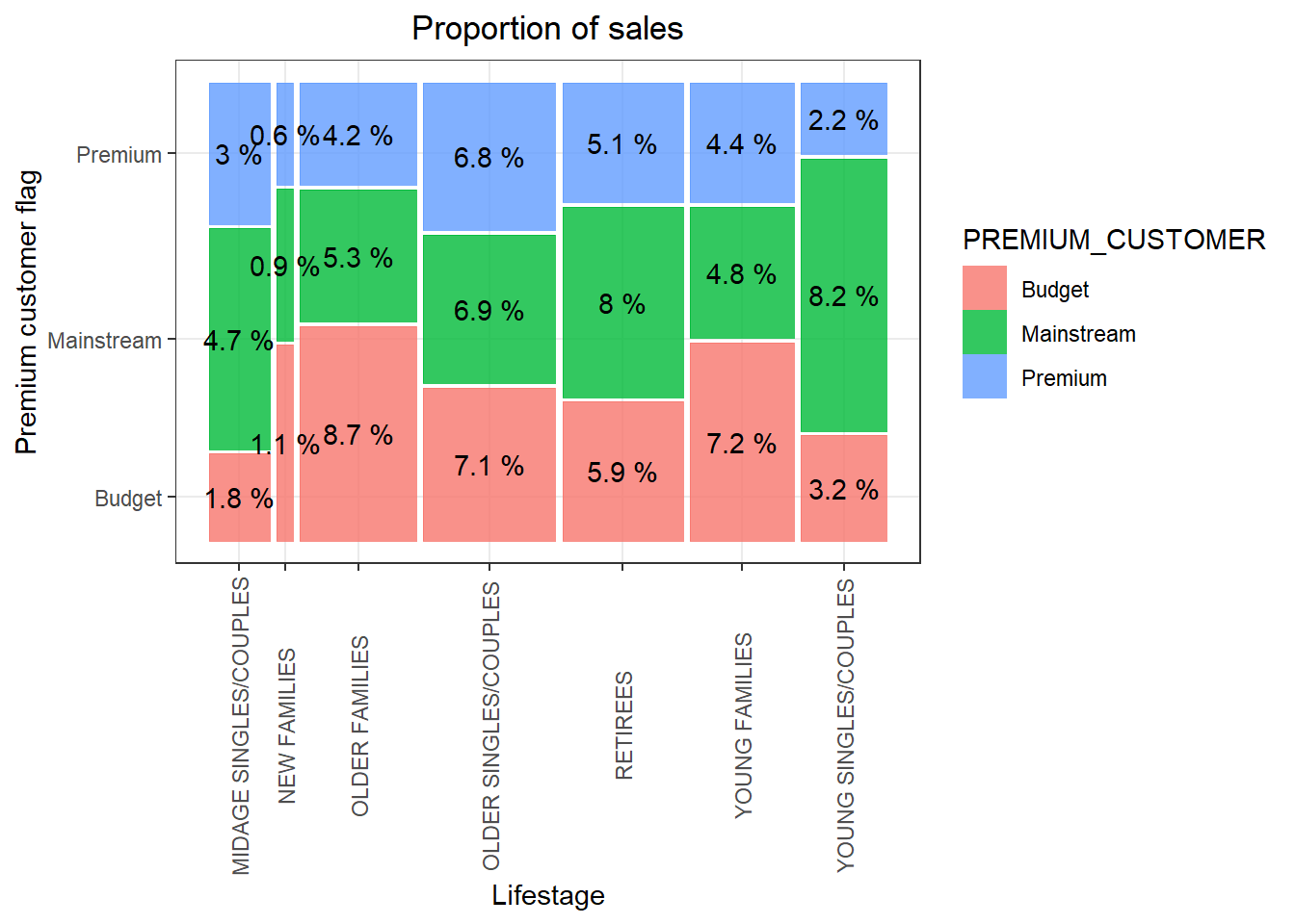
Sales are coming mainly from Budget - older families, Mainstream - young singles/couples, and Mainstream - retirees
Number of customers by LIFESTAGE and PREMIUM_CUSTOMER
Let’s see if the higher sales are due to there being more customers who buy chips.
total_sales <- data %>% group_by(LIFESTAGE,PREMIUM_CUSTOMER)

no_of_customers <- summarise(total_sales,customer_count = length(unique(LYLTY_CARD_NBR)))

summary(no_of_customers)

#### Create plot
p <- ggplot(data = no_of_customers) + geom_mosaic(aes(weight = customer_count, x = product(PREMIUM_CUSTOMER, LIFESTAGE), fill = PREMIUM_CUSTOMER)) + labs(x = "Lifestage", y = "Premium customer flag", title = "Proportion of customers") + theme(axis.text.x = element_text(angle = 90, vjust = 0.5))+ geom_text(data = ggplot_build(p)$data[[1]], aes(x = (xmin + xmax)/2 , y = (ymin + ymax)/2, label = as.character(paste(round(.wt/sum(.wt),3)*100, '%'))))


p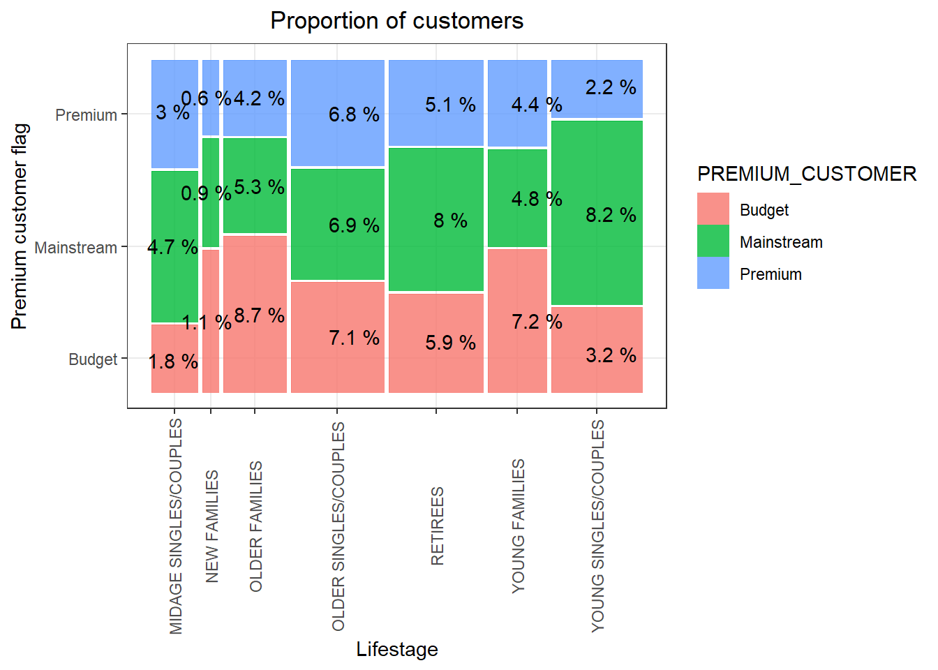
There are more Mainstream - young singles/couples and Mainstream - retirees who buy chips. This contributes to there being more sales to these customer segments but this is not a major driver for the Budget - Older families segment.
Higher sales may also be driven by more units of chips being bought per customer.
Let’s have a look at this next.
Average number of units per customer by LIFESTAGE and PREMIUM_CUSTOMER
total_sales_1 <-data %>% group_by(LIFESTAGE,PREMIUM_CUSTOMER)

units <-  summarise(total_sales_1, units_count = (sum(PROD_QTY)/uniqueN(LYLTY_CARD_NBR)))

summary(units)

###create plot
ggplot(data = units, aes(weight = units_count, x = LIFESTAGE, fill = PREMIUM_CUSTOMER)) + geom_bar(position = position_dodge()) +
labs(x = "Lifestage", y = "Avg units per transaction", title = "Units per customer") + theme(axis.text.x = element_text(angle = 90, vjust = 0.5))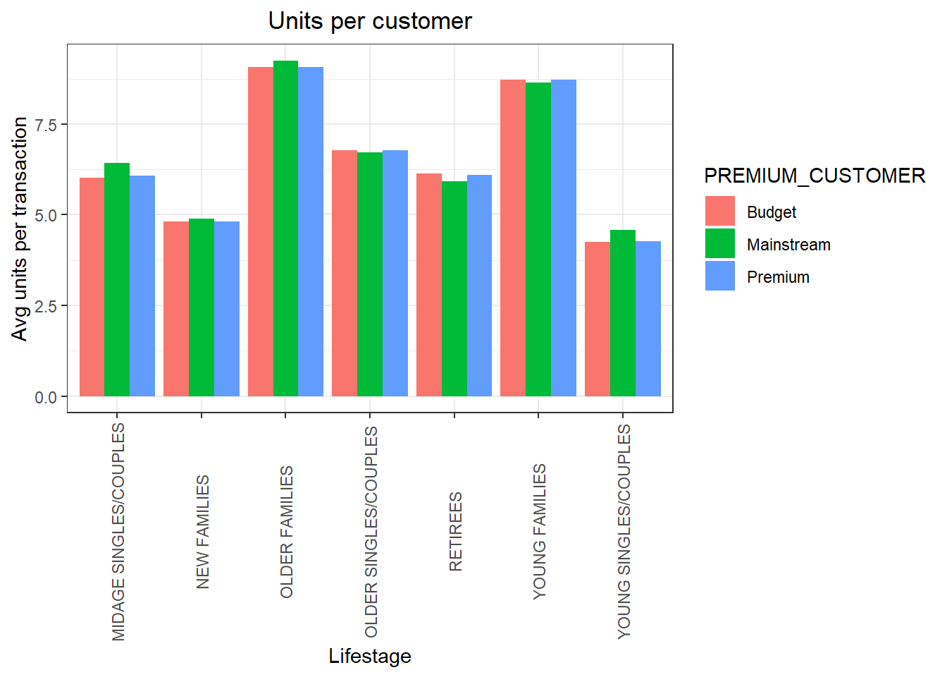
check <- units[order(units$units_count, decreasing = T),]Older families and young families in general buy more chips per customer
Average price per unit by LIFESTAGE and PREMIUM_CUSTOMER
Let’s also investigate the average price per unit chips bought for each customer segment as this is also a driver of total sales.
total_sales_2 <-data %>% group_by(LIFESTAGE,PREMIUM_CUSTOMER)

pricePerUnit <-  summarise(total_sales_2, price_per_unit = (sum(TOT_SALES)/sum(PROD_QTY)))

####plot
ggplot(data=pricePerUnit, aes(weight = price_per_unit,x = LIFESTAGE, fill = PREMIUM_CUSTOMER)) + geom_bar(position = position_dodge()) + labs(x = "Lifestage", y = "Avg price per unit", title = "Price per unit") + theme(axis.text.x = element_text(angle = 90, vjust = 0.5))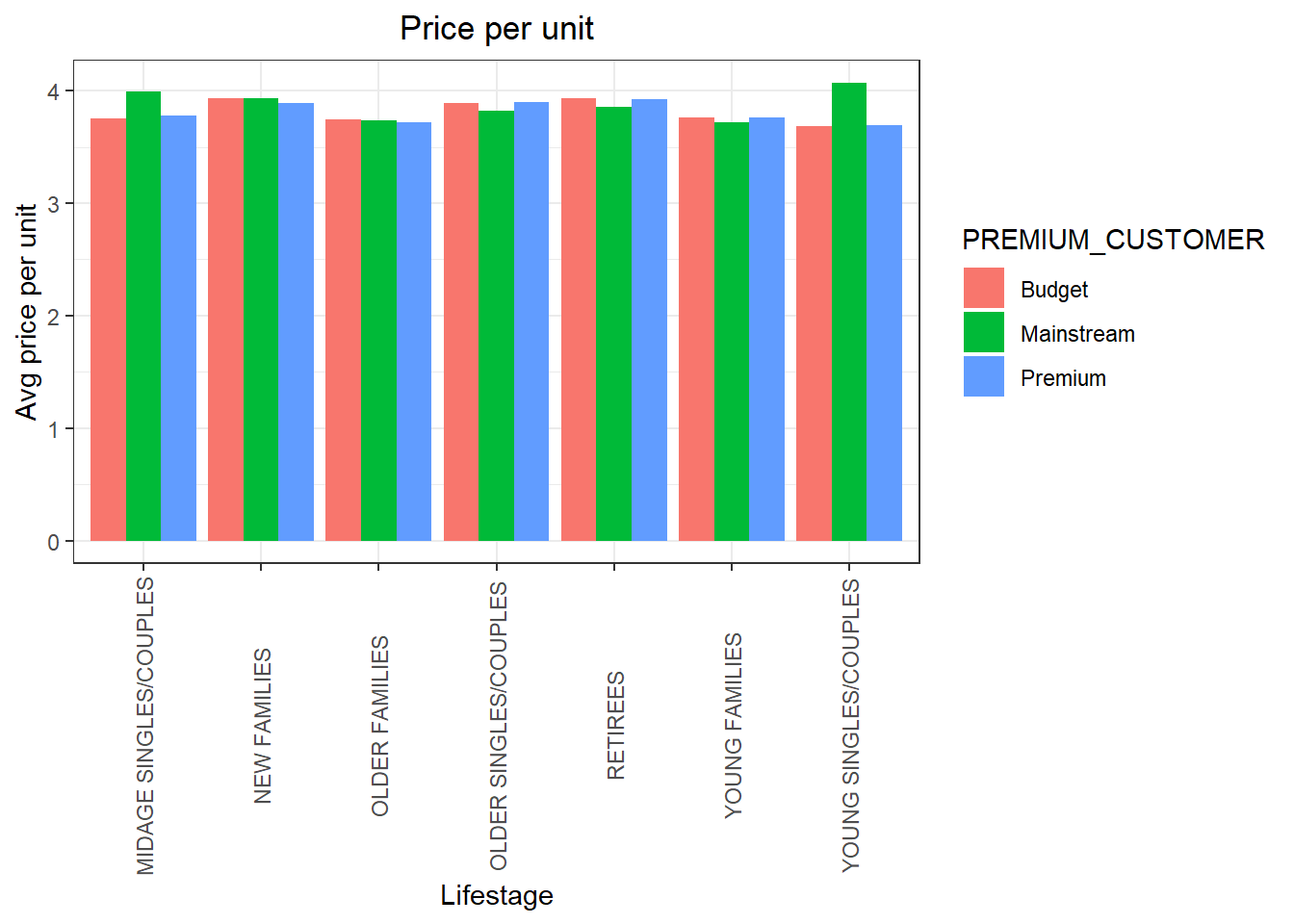
Mainstream midage and young singles and couples are more willing to pay more per packet of chips compared to their budget and premium counterparts. This may be due to premium shoppers being more likely to buy healthy snacks and when they buy chips, this is mainly for entertainment purposes rather than their own consumption. This is also supported by there being fewer premium midage and young singles and couples buying chips compared to their mainstream counterparts.
As the difference in average price per unit isn’t large, we can check if this difference is statistically different.
Deep dive into specific customer segments for insights
We have found quite a few interesting insights that we can dive deeper into. We might want to target customer segments that contribute the most to sales to retain them or further increase sales. Let’s look at Mainstream - young singles/couples. For instance, let’s find out if they tend to buy a particular brand of chips.
Deep dive into Mainstream, young singles/couples
#### Deep dive into Mainstream, young singles/couples
segment1 <- data[LIFESTAGE == "YOUNG SINGLES/COUPLES" & PREMIUM_CUSTOMER == "Mainstream",]
other <- data[!(LIFESTAGE == "YOUNG SINGLES/COUPLES" & PREMIUM_CUSTOMER =="Mainstream"),]

#### Brand affinity compared to the rest of the population
quantity_segment1 <- segment1[, sum(PROD_QTY)]

quantity_other <- other[, sum(PROD_QTY)]

quantity_segment1_by_brand <- segment1[, .(targetSegment = sum(PROD_QTY)/quantity_segment1), by = BRAND]

quantity_other_by_brand <- other[, .(other = sum(PROD_QTY)/quantity_other), by = BRAND]

brand_proportions <- merge(quantity_segment1_by_brand, quantity_other_by_brand)[, affinityToBrand := targetSegment/other]

brand_proportions[order(‐affinityToBrand)]

ggplot(brand_proportions, aes(brand_proportions$BRAND,brand_proportions$affinityToBrand)) + geom_bar(stat = "identity",fill = "yellow") + labs(x = "Brand", y = "Customers Affinity to Brand", title = "Favorite brands of Customers") + theme(axis.text.x = element_text(angle = 90, vjust = 0.5))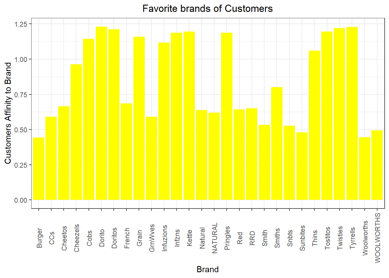
We can see that:
• Mainstream young singles/couples are 23% more likely to purchase Tyrrells chips compared to the rest of the population • Mainstream young singles/couples are 56% less likely to purchase Burger Rings compared to the rest of the population
[INSIGHTS] Let’s also find out if our target segment tends to buy larger packs of chips.
Preferred pack size compared to the rest of the population
quantity_segment1_by_pack <- segment1[, .(targetSegment = sum(PROD_QTY)/quantity_segment1), by = PACK_SIZE]

quantity_other_by_pack <- other[, .(other = sum(PROD_QTY)/quantity_other), by = PACK_SIZE]

pack_proportions <- merge(quantity_segment1_by_pack, quantity_other_by_pack)[, affinityToPack := targetSegment/other]

pack_proportions[order(‐affinityToPack)]
We can see that the preferred PACK_SIZE is 270g.
data[PACK_SIZE == 270, unique(PROD_NAME)]## [1] "Twisties Cheese 270g" "Twisties Chicken270g"Conclusion
Let’s recap what we’ve found! Sales have mainly been due to Budget - older families, Mainstream young singles/couples, and Mainstream - retirees shoppers. We found that the high spend in chips for mainstream young singles/couples and retirees is due to there being more of them than other buyers. Mainstream, midage and young singles and couples are also more likely to pay more per packet of chips. This is indicative of impulse buying behaviour.
We’ve also found that Mainstream young singles and couples are 23% more likely to purchase Tyrrells chips compared to the rest of the population. The Category Manager may want to increase the category’s performance by off-locating some Tyrrells and smaller packs of chips in discretionary space near segments where young singles and couples frequent more often to increase visibilty and impulse behaviour.
Quantium can help the Category Manager with recommendations of where these segments are and further help them with measuring the impact of the changed placement. We’ll work on measuring the impact of trials in the next task and putting all these together in the third task.
Outro
Task 1 was basic but crucial. All the basic analysis and visualizations were made here. The general patterns and trends among customers’ choices were explored through visualizations.
The solutions to the other tasks will be uploaded soon. Till then, any feedbacks, queries or recommendations are appreciated on any of my social media handles.
Refer to my Github Profile
Stay tuned for more tutorials!
Thank You!